A Bernoulli Trial xi
A Bernoulli trial is an experiment that can have only two possible outcomes
with probabilities p (of success) and q (of failure), respectively, where p + q = 1. The probabilities of those
outcomes stay constant if the same Bernoulli trial is repeated. A Bernoulli trial is denoted
as \(x_i \ \text{which can take a value of } 1 \ or \ 0\). Usually we call \(x_i = 1\) a "success";
however, this is not always a good term to use, especially in the context of clinical trials.
Suppose we count as a success getting a "6" on the toss of a die. In this case a Bernoulli trial is a
single toss, and the probability of success is p = 1/6, because landing with the "6" facing up is one of
six equally probable outcomes. Let us clarify that statement. Each Bernoulli trial
can only have one of two values, 1 or 0, respectively for success or failure. However, the probabilities
of those outcomes are not usually equal. In the case of a coin toss they are indeed equal
(\(p = q = \frac{1}{2}\)) but in the described die toss case they are not (\(p = \frac{1}{6}, \ q = 1-p =\frac{5}{6}\)).
A Binomial Random Variable X
A binomial random variable counts the number of successes in N Bernoulli trials. We express a binomial random variable as \(X\). $$X = \sum\limits_{i=1}^{n}x_i$$
The Expected Values of xi and X
Note: \(\mathbb{E}\) is the expected value operator.
The expected value of a single Bernoulli trial is p.
$$\mathbb{E}[x_i] = 1\times p + 0\times (1-p) = p$$
Therefore, the expected value in the single die toss described above (getting a "6") is:
$$\mathbb{E}[x_i] = 1\times \frac{1}{6} + 0\times\frac{5}{6} = \frac{1}{6}$$
The expected value for a binomial random variable X
is \(\mathbb{E}[X] = np\), where X is the total number of successes.
Therefore, the expected value in 60 die tosses (expected number of "6's) is:
$$\mathbb{E}[X] = np = \frac{60}{6} = 10$$
The Binomial Distribution Equation
In practice, if you look at the results of each binomial random variable, you rarely get exactly the expected outcome \(\mathbb{E}[X] = np\). Instead, you get a distribution of possible outcomes, which in theory could be any number from 0 to n, with a higher probability of getting a number close to np than a number close to 0 or n. The equation that gives you the probability of getting exactly R successes in N Bernoulli trials, where each has a probability of success p is:
\(\bbox[bisque]{P(R,p,N)= \binom{N}{R}p^R(1-p)^{(N-R)}= \frac{N!}{R!(N-R)!}p^R (1-p)^{(N-R)}}\) derivationDERIVATION: the binomial distribution equation
The probability of observing R outcomes in N Bernoulli trials is given by the Binomial or Bernoulli Distribution:
$$P(R,p,N) = \binom{N}{R} p^R (1-p)^{(N-R)} = \frac{N!}{R!(N-R)!} p^R (1-p)^{(N-R)}$$Start by asking what is the probability of having R successes (for example 3), happening in very first Bernoulli trials with the remainder trials for a total of N (for example 10) being all failures. This is what this example would look like: 1110000000. The probability of that configuration is the product: $$pppqqqqqqq = p^3q^7 = p^3(1-p)^{10-3} $$ Now if you ask what is the probability of having R successes in N trials (again 3 successes in 10 trials) you have to multiply the above probability by the number of all possible configurations: 1101000000, 1100100000, ... etc. And that is the number of combinations \(\binom{10}{3}\). More generally: $$P(R,p,N) = \binom{N}{R} p^R (1-p)^{(N-R)}$$ $$\binom{N}{R} = \text{number of combinations of R objects taken from a collection of N total objects}$$ Now let us derive the combinations formula. Imagine that your N Bernoulli trials are beans. So you have N beans. Please number them all 1 through N, place them in a box and shake the box to mix them. Now pick R beans from the box. Those are your "success" trials. Look at the numbers that you got. They were bean 41, bean 8, bean 83, ... etc up to the last bean which was number 31. Mathematically speaking, what you just did could have been done in \(N(N-1)(N-2)(N-3)...(N-R+1)\) possible ways. Because the first bean you picked (number 41) could have been any of the original N beans. The second bean (number 8) could have been any of the remaining N-1 beans and so on until (N-R+1) that last bean (number 31) was picked out of (N-R+1) leftover beans. Now multiply that number by \(\frac{(N-R)!}{(N-R)!}\), you still get the same number because that fraction equals 1, but you get it in the following form:
$$\frac{N(N-1)(N-2)(N-3)...(N-R+1)(N-R)!}{(N-R)!}=\frac{N!}{(N-R)!}$$So, these are all the possible ways in which you can draw R successes. However, there is some redundancy here, because whenever the same beans are picked that counts as just one binomial random variable. That is, if for example R=3, it does not matter if I picked beans 41, 8, and 83 in that order, or in any other order: 41, 83, 8 or 8, 41, 83. Those were the winners, regardless of the drawing order. Therefore, we have to divide our total number of possible ways to draw R successes by R!. That is the number of permutations of the same beans. So the final number of ways is:
$$\binom{N}{R} = \frac{N!}{R!(N-R)!}$$And the binomial distribution equation is thus,
$$P(R,p,N) = \binom{N}{R} p^R (1-p)^{(N-R)} = \frac{N!}{R!(N-R)!} p^R (1-p)^{(N-R)}$$Why is R! the number of permutations of R objects? To show this place R numbered beans in a box, mixed them up and draw as above. But, this time you are going all the way until you draw the last bean. You realize now that you could have done that in \(N(N-1)(N-2)(N-3)...(N-N+1) = N!\) possible ways. For example for 5 beans that is 5 x 4 x 3 x 2 x 1 = 5!.
Mean
\(\mu = np\)Variance and Standard Deviation
\(Var(X) = \mathbb{E}[(X - \mathbb{E}[X])^2]\)\(Var(X) = \sigma^2 = npq \ , \ StDev(X) = \sigma = \sqrt{npq}\)
The variance of a single Bernouli trial is \(Var(x_i) = pq\) derivation
DERIVATION: \(Var(x_i) = pq\)
Variance is defined as \(Var(x_i) = \mathbb{E}[(x_i - \mathbb{E}[x_i])^2]\)
\(\mathbb{E}[x_i^2 - 2x_i \mathbb{E}[x_i] + (\mathbb{E}[x_i])^2]\)
\(\mathbb{E}[x_i^2] - 2\mathbb{E}[x_i E[x_i]] + \mathbb{E}[(\mathbb{E}[x_i])^2]\)
\(\mathbb{E}[x_i]\) is a constant, therefore:
\(\mathbb{E}[x_i^2] - 2\mathbb{E}[x_i]E[x_i] + (\mathbb{E}[x_i])^2\)
\(\mathbb{E}[x_i^2] - 2(\mathbb{E}[x_i])^2 + (\mathbb{E}[x_i])^2\)
\(Var(x_i) = \mathbb{E}[x_i^2] - (\mathbb{E}[x_i])^2\)
\(x_i^2 = x_i\) because \(x_i\) can only be 1 or 0
\(\mathbb{E}[x_i] = p\)
Therefore \(Var(x_i) = \mathbb{E}[x_i^2] - (\mathbb{E}[x_i])^2 = p - p^2 = p(1-p) = pq\)
The variance of a binomial random variable is: \(Var(X)=\sigma^2= \sum\limits_{i=1}^{n}Var(x_i) = npq\).
This is because each Bernoulli trial (xi), is independent and therefore, we can sum their
variances to obtain the variance of a binomial random variable X. For proof see:
Normal Distribution / Proof of the Sample Variance Equation / Proof of Equality 5
Unfortunately, the same symbol \(\sigma^2\) is used for the variance of a single Bernoulli trial (xi)
and for a binomial random variable (X).
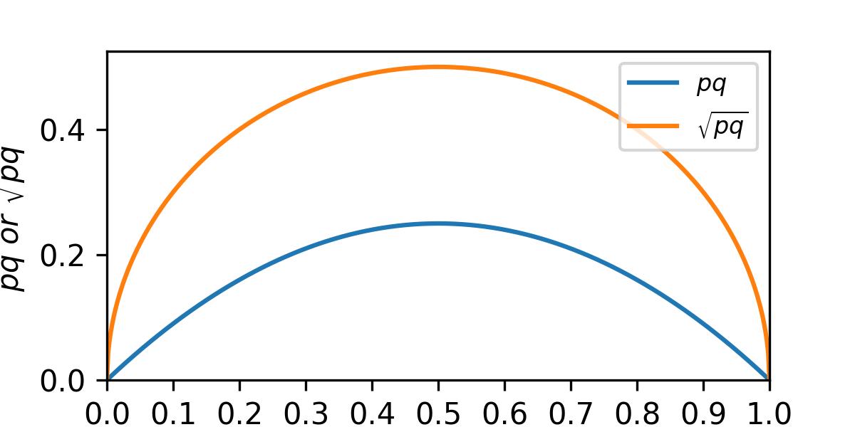
Note that both the variance and the standard deviation are greatest when p = q = 0.5 and get
smaller when either p or q approach 0 or 1 (see Figure B1).
import numpy as np
import matplotlib.pyplot as plt
p_ = np.linspace(0,1,500)
v_ = []
s_ = []
for p in p_:
    v_.append(p*(1-p))
    s_.append(np.sqrt(p*(1-p)))
fig, ax = plt.subplots(figsize=(4,2))
ax.plot(p_,v_,label=r'$pq$')
ax.plot(p_,s_,label=r'$\sqrt{pq}$')
ax.set_xlabel("p")
ax.set_ylabel(r"$pq \ or \ \sqrt{pq}$")
ax.set_xlim(left=0,right=1)
ax.set_ylim(bottom=0)
ax.set_xticks([0,0.1,0.2,0.3,0.4,0.5,0.6,0.7,0.8,0.9,1])
ax.legend(loc="upper right", fontsize=8)
plt.savefig('Know_Stats_Fig_b1.jpeg', dpi=300)
plt.show()
The Sample Proportion \( \ \hat{p} \ \) and its Variance
Suppose you throw the die 60 times and count the wins as 12.
Then, \(\hat{p} = \frac{12}{60} = 0.20\) is called a sample proportion.
$$\hat{p} = \frac{\sum\limits_{i=1}^{n}x_i}{n} = \frac{X}{n}$$
Recall that \( \sum\limits_{i=1}^{n}x_i\) will be something like: 0 + 1 + 0 + 0 + 1 + ... etc.
The variance of a sample proportion is:
The formulas for the "standard deviation" and "standard error of the sample proportion" are identical, so, why not use just one of the terms? The standard deviation \(\sigma\) is a true population parameter, but it is most frequently unknown, thus, we use the term "standard error" \(SE(\hat{p})\) to emphasize that it is an estimate. $$ \sigma = \sqrt{\frac{p(1-p)}{n}} \text{ where p is the true population proportion}$$ $$ SE(\hat{p}) = \sqrt{\frac{\hat{p}(1 - \hat{p})}{n}} \ where \ \hat{p}\text{ is an estimate of } p$$
The Moment Generating Function (MFG) and its First Four Moments: Mean, Variance, Skewness, and Kurtosis
Moment Generating Function \( \ M(t) = (q + pe^t)^n\) derivationMoment Generating Function of the Binomial Distribution
A moment generating function is defined as: \(M_X(t) = \mathbb{E}[e^{tX}]\)
where
- X is a random variable (for the binomial distribution, X takes integer values k = 0, 1, ..., n)
- t is a real number (for example when calculating the 2nd moment, which is the variance, we take the derivative of \(M_X(t)\) and evaluate it at t = 0)
\(\mathbb{E}[e^{tX}]\) is the expectation or the mean of all possible values of \(e^{tX}\). Therefore, if X can take any 0, or positive integer value k = 0, 1, 2,...n, then \( \ \mathbb{E}[e^{tX}] \ \) is the sum of all possible values of \( \ e^{tk} \ \), each multiplied by its probability, that is:
$$ M_X(t) = \mathbb{E}[e^{tX}] = \sum_{k=0}^n e^{tk} \mathbb{P}(X = k) $$For a binomial random variable \( \ \mathbb{P}(X = k) = \binom{n}{k} p^k (1 - p)^{n - k}\)
Therefore:\( \ M_X(t) = \sum\limits_{k=0}^{n} e^{tk} \binom{n}{k} p^k (1 - p)^{n - k} = \sum\limits_{k=0}^{n} \binom{n}{k} \left(p e^t\right)^k (1 - p)^{n - k}\)
Recalling the binomial expansion:
\((a+b)^n =\binom{n}{0}a^nb^0 + \binom{n}{1}a^{n-1}b^1\dots+\binom{n}{n}a^{0}b^n = \sum\limits_{k=0}^{n}
\binom{n}{k}a^{n-k}b^{k}\)
we define \(b = p e^t \ and \ a = 1 - p = q\), and thus, rewrite the equation as:
Mean \( \ \mu = np\) derivation
The mean \( \ (\mathbb{E}[X]) \ \)is the first moment of the MGF; therefore, we take the first derivative of the MFG and evaluate it at k = 0.
- \(\frac{dM(t)}{dt}= n(q + pe^t)^{n-1}pe^t\)
- \(\mu = \frac{dM(t)}{dt}|_{t=0} = np(q + p)^{n-1} = np(1 - p + p)^{n-1} = np\)
Variance \( \ \sigma^2 = npq\) derivation
Variance \(\sigma^2 = \mathbb{E}[X^2] - \mathbb{E}[X]^2\) where \(\mathbb{E}[X^2] \ \)is the second moment of the MGF , which we obtain by taking the second derivative of the MFG and evaluating it at k = 0. We already evaluated \(\mathbb{E}[X]\), which is the mean.
- \(\frac{dM(t)}{dt}= n(q + pe^t)^{n-1}pe^t\)
- \(\frac{d^2M(t)}{dt^2}= n(n-1)(q + pe^t)^{n-2}p^2e^{2t} + n(q + pe^t)^{n-1}pe^t \)
- \(\frac{d^2M(t)}{dt^2}|_{t=0} = n(n-1)(q + p)^{n-2}p^2 + n(q + p)^{n-1}p\)
- because q + p = 1, the above equation simplifies to:
- \(n(n-1)p^2 + np = np(np-p+1) = np(np + q) = (np)^2 + npq \)
- \(\sigma^2 = \mathbb{E}[X^2] - \mathbb{E}[X]^2 = (np)^2 + npq - (np)^2 = npq\)
Skewness \( \ \alpha_3 = \frac{q - p}{\sqrt{npq}}\) derivation
skewness\( \ \alpha_3 = \frac{\mathbb{E}[X^3] - 3\mu\sigma^2 - \mu^3}{\sigma^3} \ \) where \( \ \mathbb{E}[X^3] \ \) is the third moment of the MGF , which we obtain by taking the third derivative of the MFG and evaluating it at k = 0.
- \(\frac{dM(t)}{dt}= n(q + pe^t)^{n-1}pe^t\)
- \(\frac{d^2M(t)}{dt^2}= n(n-1)(q + pe^t)^{n-2}p^2e^{2t} + n(q + pe^t)^{n-1}pe^t \)
- \(\frac{d^3M(t)}{dt^3}= n(n-1)(n-2)(q + pe^t)^{n-3}p^3e^{3t} + \)
\(3n(n-1)(q + pe^t)^{n-2}p^2e^{2t} + n(q + pe^t)^{n-1}pe^t\) - p+q = 1, therefore: \( \ \frac{d^3M(t)}{dt^3}|_{t=0} = n(n-1)(n-2)p^3 + 3n(n-1)p^2 + np\)
-
Substitute the known expressions into the skewness formula:
\( \text{Skewness} = \frac{ n(n{-}1)(n{-}2)p^3 + 3n(n{-}1)p^2 + np - 3np(npq) - (np)^3 }{(npq)^{3/2}} = \) - \( \frac{n(n{-}1)(n{-}2)p^3 + 3n(n{-}1)p^2 + np - 3n^2p^2q - n^3p^3}{(npq)^{3/2}} \)
- \(\frac{n^3p^3 - 3n^2p^3 +2np^3 + 3n^2p^2-3np^2 + np - 3n^2p^2q - n^3p^3}{(npq)^{3/2}} =\)
- \(\frac{- 3n^2p^3 +2np^3 + 3n^2p^2-3np^2 + np - 3n^2p^2q}{(npq)^{3/2}} =\)
- \(\frac{np(- 3np^2 +2p^2 + 3np-3p - 3npq + 1)}{(npq)^{3/2}} = \)
- \(\frac{np(- 3np^2 +2p^2 + 3np-3p - 3np(1-p) + 1)}{(npq)^{3/2}} = \)
- \(\frac{np(-3np^2 +2p^2 + 3np-3p - 3np+3np^2 + 1)}{(npq)^{3/2}} = \)
- \(\frac{np(2p^2-3p+ 1)}{npq\sqrt{npq}} = \)
- \(\frac{(2p^2-3p+ 1)}{q\sqrt{npq}} = \)
- \(\frac{2(1-q)^2-3p+ 1}{q\sqrt{npq}} = \)
- \(\frac{2-4q +2q^2-3p+ 1}{q\sqrt{npq}} = \)
- \(\frac{3 - 3p -4q +2q^2}{q\sqrt{npq}} = \)
- \(\frac{3(1- p) -4q +2q^2}{q\sqrt{npq}} = \)
- \(\frac{-q +2q^2}{q\sqrt{npq}} = \)
- \(\frac{2q-1}{\sqrt{npq}} = \frac{q + q -1}{\sqrt{npq}} = \frac{q + 1 - p -1}{\sqrt{npq}}=\)
- \(\frac{q - p}{\sqrt{npq}}\)
Kurtosis
\(\alpha_4 = 3 + \frac{1 - 6pq}{\sqrt{npq}}\)Comparison of the Normal and the Binomial Distributions
Figure B2 shows superimposed examples of a binomial and a normal distribution. As you can see, they do not superimpose perfectly. That is because p and q are different, which introduces a skewness to the binomial distribution relative to the "perfect" normal distribution. Regardless, we can use the same concepts described for the normal distribution to calculate confidence intervals. The real life examples described in the next section show you how to do that.
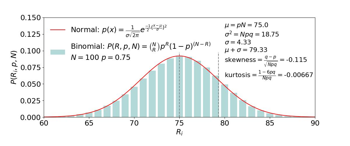
The following Python code was used to make the figure including the calculation of the mean, the variance, the skewness, and the kurtosis given the initial parameters (N =100 and p = 0.75).
Fig B2 Python Code
import numpy as np
import matplotlib.pyplot as plt
import math
from scipy.stats import norm
from scipy.stats import binom
N = 100
p = 3/4
q = 1-p
mu,v,sk,k = binom.stats(N,p,moments="m,v,s,k")
s = math.sqrt(v)
R_ = list(range(N+1))
PofR_ = binom.pmf(R_,N,p)
x_ = np.linspace(55,95,300)
ynorm_ = norm.pdf(x_,mu,s)
fig, ax = plt.subplots(figsize=(12,5))
# TITLE, LEGEND AND OTHER ANNOTATIONS
ax.tick_params(axis='both', which='major', labelsize=18)
ax.text(80,0.06, r'$\mu = pN = $'+ f'{mu:.4}' + '\n' +
r'$\sigma^2 = Npq = $' + f'{v:.4}' + '\n' +
r'$\sigma =$' + f'{s:.3}'  + '\n' +
r'$\mu + \sigma =$' + f'{mu+s:.2f}' + '\n' +
r'$\text{skewness} = \frac{q-p}{\sqrt{Npq}} =$' + f'{sk:.3}' + '\n' +
r'$\text{kurtosis} = \frac{1-6pq}{Npq}=$' + f'{k:.3}',fontsize=16)
# AXES
ax.set_xlabel(r'$R_i$',fontsize=18)
ax.set_ylabel(r'$P(R_i,p,N)$',fontsize=18)
ax.set_xlim(left=60, right=90)
ax.set_ylim(bottom=0, top=0.15)
# PLOT
ax.axvline(x=mu, color='grey', linestyle='--',ymax=0.65)
ax.axvline(x=mu + s, color='grey', linestyle='--', ymax=0.65)
ax.bar(R_, PofR_, color='teal', alpha=.3, label=r'$\text{Binomial:} \ P(R,p,N)= \binom{N}{R}p^R(1-p)^{(N-R)}$' + f'\n' + r'$N=100 \ p=0.75$')
ax.plot(x_, ynorm_, linestyle="-", marker="none", color='red', label=r'$\text{Normal:} \ p(x)=\frac{1}{\sigma\sqrt{2\pi}}e^{\frac{-1}{2}{(\frac{x-\mu}{\sigma})}^{2}}$')
ax.legend(loc="upper left", frameon=False,fontsize=18)
plt.show()
Example from the Real World
The following cancer mortality numbers were from taken from the CDC.
Year: 2021 State:CA Sex:male Race:white Ethnicity:non-hispanic. Age:70-74 #Deaths:290 Population:422,747 CrudeRate (deaths/100,000):68.599 95%CI: 60.930 - 76.966 StdErr:4.028
Our calculations:
$$\hat{p}=\frac{290}{422,747} \approx 0.00068599 = \frac{68.599}{100,000}$$ $$SE = \frac{\sqrt{p(1-p)}}{n} \ where \ p=\mathbb{E}[p] = \hat{p}$$ $$SE = \frac{\sqrt{0.00068599(1-0.00068599)}}{422,747}\approx 0.0000402689 = \frac{4.027}{100,000}$$ $$use \ z=1.96 \ \text{for a 2-tail 95% c.i.}$$ $$68.599-1.96 \times 4.028 \lt \text{95%c.i.} \lt 68.599 + 1.96 \times 4.028 \rightarrow 60.704 \ - \ 76.494$$The slightly different c.i. numbers that we obtained are probably explained by the CDC having used the Poisson distribution. The Poisson distribution is special case of the binomial distribution. We will describe it in the next section.