Definition, Equation Derivation, and Example
Everyone has heard of a bell curve and has a general idea of what it is. Bell curves, regardless of their exact shape, are described by the normal distribution (aka "Gaussian distribution") equation, normalized to the number of individuals in the studied population. The normal distribution is a continuous probability density function (PDF) that is symmetrical around the mean. The normal distribution equation describes the probability of observing a value x, in a population with a mean \(\mu\) and a standard deviation \(\sigma\) (variance = \(\sigma^2\)).
The Normal Distribution Equation: \(\bbox[bisque]{\ p(x)=\frac{1}{\sigma\sqrt{2\pi}}e^{\frac{-1}{2}{(\frac{x-\mu}{\sigma})}^{2}}}\) derivationDerivation of the normal distribution equation
I am, more or less, following the derivation posted on this web page , by Dan Teage, but will explain in more detail some of the steps that might not be obvious to non-mathematicians.
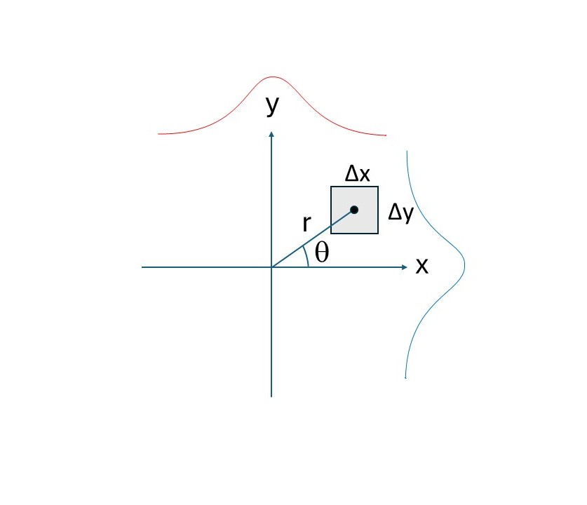
Figure N1 represents a point in an x, y cartesian coordinates space such that: the probability of finding it in a region with area \(\Delta\)x\(\Delta\)y, at distance r from the origin fits the following criteria:
- it is a positive number
- it is independent of the angle \(\theta\)
- it is proportional to the area of the square \(\Delta\)x\(\Delta\)y
- it decreases as r increases
- the sum of all probabilities is exactly 1
The following equation satisfies the above criteria: $$f(x)\Delta xf(y)\Delta y = g(r)\Delta x\Delta y$$ The f(x) is the probability of finding a point at a distance x from the y axis and vice-versa for f(y). Importantly, it is the same function for both the x and the y variables. Multiplying f(x) by f(y) yields a result that is consistent with our criteria. For example, \(f(x=1)\dot f(y=1) > f(x=1)\dot f(y=10)\). On the right side of the equation we have a different function that is also consistent with the criteria. For example,\( \ g(r=1)\dot > g(r=10)\). If we project all possible points along the x-axis or the y-axis, the densities of their projections are, respectively f(x) and f(y), which are both normal distributions with the same \(\mu\) and \(\sigma^2\) parameters. Figure N1 illustrates this, where the blue and red curves are the normal distributions for x and y, respectively.
The above equation simplifies to: $$f(x)f(y)=g(r)$$ Since the probability is independent of \(\theta\), that is, the expression is invariant under rotation, we can write: $$\frac{d[f(x)f(y)]}{d\theta} = 0$$ $$\text{Expand and substitute in} \ x = rcos(\theta) \ and \ y = rsin(\theta).$$ $$f^{'}(x)\frac{drcos(\theta)}{d\theta}f(y) + f(x)f^{'}(y)\frac{drsin(\theta)}{d\theta} = $$ $$f^{'}(x)(-rsin(\theta))f(y) + f(x)f^{'}(y)rcos(\theta) = 0$$ $$xf(x)f^{'}(y) = f^{'}(x)yf(y)$$ $$\frac{f^{'}(y)}{yf(y)} = \frac{f^{'}(x)}{xf(x)}$$ If two expressions are equal for any x and y, (the key word here is "any") it implies that they are equal to some constant value. So, let us solve one of these differential equations (the other will be solved in the same way): $$\frac{f^{'}(y)}{yf(y)} = k \rightarrow \frac{f^{'}(y)}{f(y)} = ky \rightarrow \int \frac{f^{'}(y)}{f(y)}dy = \int kydy$$ $$ln(f(y)) = k\frac{1}{2}y^2+C\rightarrow f(y) = e^{k\frac{1}{2}{y^2}+C}= e^{C}e^{k\frac{1}{2}{y^2}} = Ae^{\frac{ky^2}{2}}$$ f(x) is the same and it is the basic form of the normal distribution equation. $$f(x) = Ae^{\frac{kx^{2}}{2}}$$ By the above criteria the integral of f(x) from \(-\infty\) to \(+\infty\) is 1. This means that k must be negative, because otherwise the integral would be infinite. Next, rewrite k as -m and figure out what A and m are. We will need to use a couple of mathematical tricks. First, let us look at the figure again and realize two things: (a) the means for both f(x) and f(y) are 0, and both the curves are symmetrical around the mean. Therefore, if we restrict ourselves to the first quadrant (x and y both 0 or positive), the integral of each function will be 1/2. In polar coordinates the positive x and y spaces correspond to 0 to \(\pi\)/2. Now, let us multiply the integral of f(x) by the integral of f(y) in the first quadrant: $$A^2\int_{0}^{\infty}e^{\frac{-m}{2}x^2}dx \int_{0}^{\infty}e^{\frac{-m}{2}y^2}dy = (\frac{1}{2})(\frac{1}{2}) = \frac{1}{4}$$ Now comes the first math trick: we can write the product of the two integrals as a double integral and combine their respective expressions. Fubini's theorem makes this possible. $$A^2\int_{0}^{\infty}\int_{0}^{\infty}e^{\frac{-m}{2}(x+y)^2}dxdy = \frac{1}{4}$$ The second trick is to convert the double integral to polar coordinates. $$A^2\int_{0}^{\frac{\pi}{2}}\int_{0}^{\infty}e^{\frac{-m}{2}r^2}rdrd\theta = \frac{1}{4}$$ To do the cartesian-polar transformation we need to calculate its Jacobian determinant (Jacobian).
$$x = rcos(\theta) \ and \ y = rsin(\theta)$$ $$\frac{dx}{dr}=cos(\theta),\frac{dy}{dr}=sin(\theta),\frac{dx}{d\theta}=-rsin(\theta),\frac{dy}{d\theta}=rcos(\theta)$$
$$The \ Jacobian \ of \ \frac{d(x,y)}{d(r,\theta)} = \begin{vmatrix} \frac{dx}{dr} & \frac{dx}{d\theta} \\ \frac{dy}{dr} & \frac{dy}{d\theta} \end{vmatrix} = \begin{vmatrix} cos(\theta) & -rsin(\theta) \\ sin(\theta) & rcos(\theta) \end{vmatrix}$$ $$cos(\theta)rcos(\theta)-sin(\theta)(-rsin(\theta)) = r(cos(\theta)^2+sin(\theta)^2) = r$$
Thus, dxdy transforms to rdrd\(\theta\), because dr must be multiplied by the Jacobian (r) for this transformation. Figure N2 should help you understand this intuitively. The blue and peach areas are infinitesimally small. The cartesian area is simply dxdy but the polar area is dr times
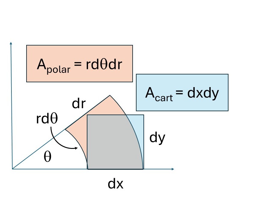
Figure N2
Next, solve the inner integral by using "integration by substitution".
$$A^2\int_{0}^{\frac{\pi}{2}}\int_{0}^{\infty}e^{\frac{-m}{2}r^2}rdrd\theta = \frac{1}{4}$$
Let U = (1/2)mr2, then du/dr = mr, du/m = rdr, substituting into the integral above:
$$\int_{0}^{\frac{\pi}{2}}\int_{0}^{\infty}e^{-U}dUd\theta = \frac{m}{4A^2}$$
Calculate the inner integral first (=1), and then outer (=\(\frac{\pi}{2}\))
$$-\frac{1}{e^\infty} - (-\frac{1}{e^0} ) = 0 + 1 = 1$$
$$ \int_{0}^{\frac{\pi}{2}}d\theta = \frac{m}{4A^2} \rightarrow \frac{\pi}{2} =\frac{m}{4A^2}$$
$$A = \sqrt{\frac{m}{2\pi}}$$
Substitute into what we called the "the basic function" above, except that we renamed k into m.
$$f(x)=\sqrt{\frac{m}{2\pi}}e^{-\frac{m}{2}x^2}$$
This is closer the the final form of the normal distribution equation,
but we still need to figure out what m is (in terms of the mean and variance).
The mean \(\mu\) is zero because of the way we derived the equation.
The variance \(\sigma^2\) can be determined by plugging in the derived equation into the
definition of variance:
$$\sigma^2=\int_{-\infty}^{+\infty}{(x-\mu)^2f(x)dx} \rightarrow (\mu=0) \rightarrow \sigma^2=\int_{-\infty}^{+\infty}{x^2f(x)dx}$$
$$\sigma^2=\sqrt{\frac{m}{2\pi}}\int_{-\infty}^{+\infty}{xxe^{-\frac{m}{2}x^2}dx}$$
Now we use another math trick called "integration by parts"
$$(uv)' = u'v + uv' \rightarrow uv' = (uv)' - u'v \rightarrow \int uv' = uv - \int u'v$$
I prefer this equivalent notation:
$$d(uv) = vdu + udv \rightarrow udv = d(uv) - vdu \rightarrow \int udv = uv - \int vdu$$
$$Let \ dv=xe^{-\frac{m}{2}x^2} \ and \ u=x \rightarrow du = 1 \ and \ v =-\frac{1}{m}e^{-\frac{m}{2}x^2}$$
$$Then \ \ \sqrt{\frac{m}{2\pi}}\int_{-\infty}^{+\infty}{xxe^{-\frac{m}{2}x^2}dx} =$$
$$\sqrt{\frac{m}{2\pi}}(x)(\frac{-1}{m})e^{-\frac{m}{2}x^2}\Biggr|_{-\infty}^{+\infty} - (\frac{-1}{m})\int_{-\infty}^{+\infty}\sqrt{\frac{m}{2\pi}}e^{-\frac{m}{2}x^2}dx$$
The integral on the right side is 1 because it is the sum of all probabilites of the normal distribution.
$$\sigma^2 = \sqrt{\frac{m}{2\pi}}(x)(\frac{-1}{m})e^{-\frac{m}{2}x^2}\Biggr|_{-\infty}^{+\infty} + (\frac{1}{m})$$
$$\sqrt{\frac{m}{2\pi}}(x)(\frac{-1}{m})e^{-\frac{m}{2}x^2}\Biggr|_{-\infty}^{+\infty} = 0 \ because \ \lim_{x \to +/-\infty}\frac{1}{e^{\frac{m}{2}x^2}} = 0$$
$$\sigma^2 = \frac{1}{m} \rightarrow m = \frac{1}{\sigma^2}$$
$$f(x) = \frac{1}{\sigma\sqrt{2\pi}}e^{-\frac{1}{2}(\frac{x}{\sigma})^2}$$
Finally we can introduce the mean \(\mu\) into the equation by means of a horizontal shift.
$$f(x) = \frac{1}{\sigma\sqrt{2\pi}}e^{-\frac{1}{2}(\frac{x-\mu}{\sigma})^2}$$
- the mean, median, and mode are all equal in a normal distribution
- the standard deviation (or its square, the variance) is the measure of the spread of the graph
- In a PDF the probability of an observation p(x) is always positive
- In a PDF of all probabilities in a given interval adds up to 1
- For the normal distribution the sum of all probabilities from \(-\infty\) to \(+\infty\) equals 1.
$$\int_{- \infty}^{+\infty}{\frac{1}{\sigma\sqrt{2\pi}}e^{\frac{- 1}{2}{(\frac{x - \mu}{\sigma})}^{2}}dx = 1\ \ }$$ $$\text{ The Sum of All Probabilities}$$
import matplotlib.pyplot as plt
import numpy as np
from scipy.stats import norm

dataFile1 = "data_heightMen.txt"
dataFile2 = "data_heightWomen.txt"

nmbrBins = 20

with open(dataFile1, "r") as f1:
   data1 = [float(line.strip()) for line in f1]
with open(dataFile2, "r") as f2:
   data2 = [float(line.strip()) for line in f2]

[counts1, bins1, patches1] = plt.hist(data1, color="blue", ec="black", alpha=0.5, bins=nmbrBins)
[counts2, bins2, patches2] = plt.hist(data2, color="red", ec="black", alpha=0.5, bins=nmbrBins)

tot1 = sum(counts1)
tot2 = sum(counts2)

m1, s1 = norm.fit(data1)
m2, s2 = norm.fit(data2)

x1 = min(min(data1), min(data2))
x2 = max(max(data1), max(data2))
x = np.linspace(x1, x2, 200)
y1 = norm.pdf(x, m1, s1) * tot1
y2 = norm.pdf(x, m2, s2) * tot2

plt.plot(x, y1, color="blue", label='men')
plt.plot(x, y2, color="red", label='women')
plt.xlabel('inches')
plt.ylabel('number')
plt.title('US Men and Women Height Distributions')

ypos = max(max(y1), max(y2))
plt.text(x1, ypos, f'tot: {tot1:.0f}m {tot2:.0f}w', fontsize=9, color='black')
plt.text(x1, ypos-4, f'mean: {m1:.1f}  {m2:.1f}', fontsize=9, color="black")
plt.text(x1, ypos-8, f'stdev: {s1:.2f}  {s2:.2f}', fontsize=9, color="black")
plt.legend()
plt.show()
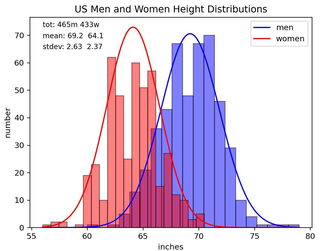
The histograms in Figure N3 are superimposed with corresponding normal distribution curves. Actually, you can't fit the data to a normal distribution equation because, obviously, the men's and women's sample sizes are greater than one. Since the total area under a normal distribution curve is 1, if we want to fit the histograms to a normal distribution, we need to normalize it to the sample size, which amounts to multiplying the PDF by the respective sample sizes (n).
$$y=n\frac{1}{\sigma\sqrt{2\pi}}e^{\frac{- 1}{2}{(\frac{x-\mu}{\sigma})}^{2}}$$ $$\text{Normalizing to the Sample Size}$$ Alternatively, one can normalize the histogram at the python code level by adding the parameter "density = True" to the plt.hist() function. We also need to plug \(\mu\) and \(\sigma\) into the PDF equation. If those values are unknown they can be calculated by fitting the PDF to the data, which is actually what we did (see the Python code that generated the figure right after the legend - data not included). Before we look at the definitions of the mean \(\mu\) and variance \(\sigma^2\) (the standard deviation is \(\sigma\) ), we must distinguish between a population and a sample. We usually don't have data for the entire population; rather, we have a sample or samples of the population from which we are trying to estimate, within a defined confidence interval, population parameters such as its mean and standard deviation.
Confidence Intervals
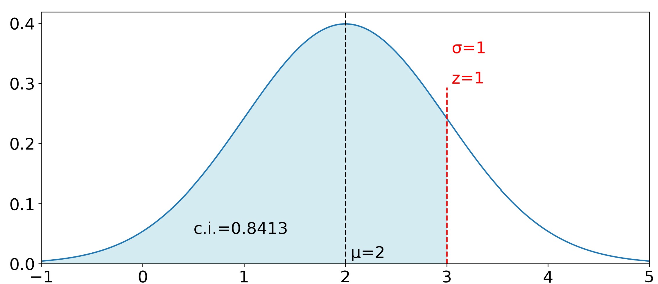
The probability of a random observation falling within an interval \( x_1 \rightarrow x_2 \) is called a confidence interval. For the normal distribution it is equal to the area under the curve, or the integral: $$\int_{x_1}^{x_2}\frac{1}{\sigma\sqrt{2\pi}}e^{-\frac{1}{2}\left( \frac{x-\mu}{\sigma}\right)^2}dx$$ $$\text{Confidence Interval}$$ This is a non-elementary integral, but approximated numerical solutions can be obtained by using power series methods. Before computers, people used tables of pre-calculated confidence intervals. These tables are still used today because for many people they are simpler to understand than computer programs. Typically, these tables (e.g., https://z-table.com/) give you the cumulative confidence interval, which is calculated using the cumulative distribution function: CDF. Mathematically this is the integral, or the area under curve, from \(-\infty \ to \ x\). Note however that you do not input x, but rather the z-score (z) which you calculate as follows: \(z=\frac{(x-\mu)}\sigma{}\). There is a very good reason to use z-scores rather than x. It is because this way you only a single number z to look up in the table, rather than 3 numbers (\(x, \ \mu, \sigma\)) in all sorts of combinations. Therefore, the CDF is more commonly stated as: $$ \text{CDF}(z) = \Phi(z) = \frac{1}{\sqrt{2\pi}} \int_{-\infty}^{z} e^{-\frac{1}{2} t^2} \, dt $$ $$\text{Cumulative Distribution Function (CDF)}$$ Here is a quick derivation of what we just did: $$ \text{Start with the integral of the normal distribution:} \ \frac{1}{\sigma \sqrt{2\pi}} \int_{-\infty}^{x} e^{-\frac{1}{2} \left( \frac{x - \mu}{\sigma} \right)^2} \, dx $$ $$ Substitute \ z = \left( \frac{x - \mu}{\sigma} \right) \Rightarrow \frac{dz}{dx} = \frac{1}{\sigma} \Rightarrow dx = \sigma \, dz$$ $$\text{The upper integral limit} \ x \ becomes \ z = \left( \frac{x - \mu}{\sigma} \right) \text{or simply} \ z$$ $$ \Phi(z) = \frac{1}{\sqrt{2\pi}} \int_{-\infty}^{z} e^{-\frac{1}{2} z^2} \, dz $$ But there is a confusing notation in the formula above. The \( z \) value in the upper limit of the integral is a constant corresponding to the \( x \) value that delimits our confidence interval, whereas the \( z \) inside the integral is a variable that can take any real number value \( x \in \mathbb{R} \). Therefore, in order to avoid this confusion, we change the name of the variable inside the integral from \( z \) to \( t \), which, of course, makes no difference mathematically. $$\bbox[bisque]{\Phi(z) = \frac{1}{\sqrt{2\pi}} \int_{-\infty}^{z} e^{-\frac{1}{2} t^2} \, dt}$$ $$\text{Cumulative Distribution Function (CDF)}$$ As an example, Figure 4 illustrates a distribution with \(\mu\) = 2 and \(\sigma\) = 1. The following are 5 different ways one can ask the same question:
- how likely is it that a random observation will be a number smaller than 3?
- what is the probability that a random observation will yield a number smaller than 3?
- what is the confidence interval for x < 3?
- what is the area under the curve from \(-\infty\) to 3?
- given that the z-value corresponding to 3 is \(\frac{3-2}{1}=1\ ,what \ is \ \Phi(1) \ or \ cdf(1)\)?
  import numpy as np
  import matplotlib.pyplot as plt
  import scipy.stats as stats
  m = 2
  s = 1
  x = np.linspace(-1,5,200)
  y = stats.norm.pdf(x,m,s)
  x_fill = np.linspace(-1,3,200)
  y_fill = stats.norm.pdf(x_fill,m,s)
  ci=stats.norm.cdf(1)
  fig,ax= plt.subplots(figsize=(12,5))
  ax.plot(x,y)
  ax.axvline(2,color='black',linestyle='--')
  ax.axvline(3,color='red',linestyle='--',ymin=0, ymax=0.7)
  ax.tick_params(axis='both',which='major',labelsize=18)
  ax.text(2,0.01,' μ=2',fontsize=18, color='black')
  ax.text(3,0.35,' σ=1',fontsize=18, color='red')
  ax.text(3,0.30,' z=1',fontsize=18, color='red')
  ax.text(0.5,0.05,f'c.i.={ci:.4f}',fontsize=18, color='black')
  ax.fill_between(x_fill,y_fill,color='lightblue',alpha=0.5)
  ax.set_ylim(bottom=0)
  ax.set_xlim(left = -1, right = 5)
  plt.show()
Looking up Z = 1 on the table (https://z-table.com/) you see that the confidence interval cdf is 0.8413. If you prefer using computer programs you can make the same calculation with Python by using the stats.norm.cdf() method. If you click the arrow below you will see the Python code that generated Figure N4. Line 10, ci=stats.norm.cdf(1), defines the variable ci = 0.8413 as the confidence interval for Z = 1.
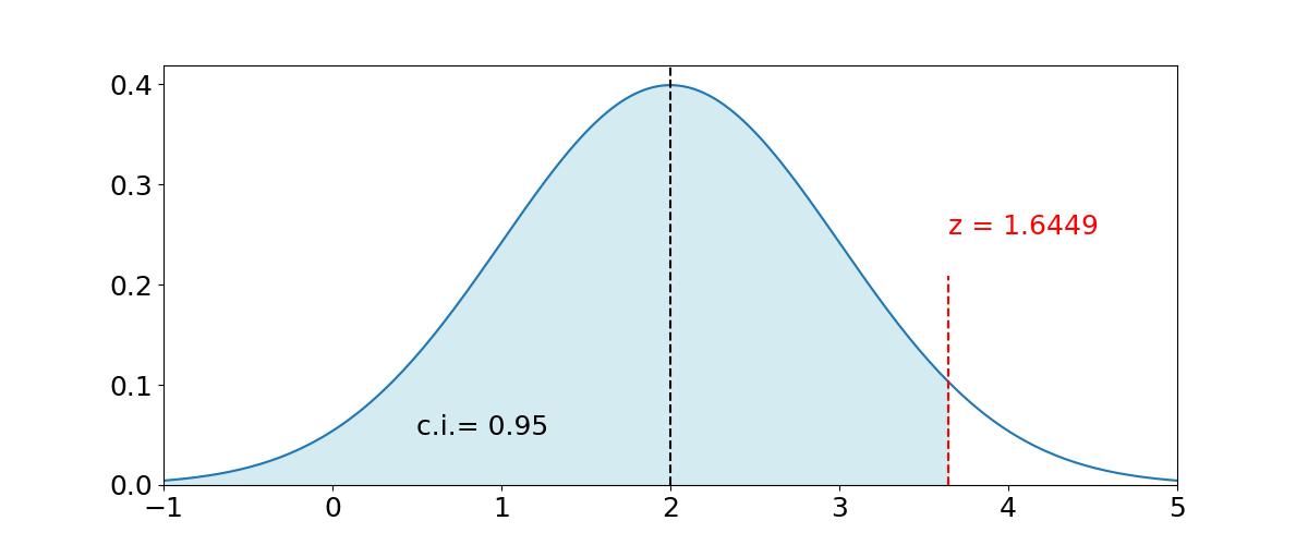
Now suppose you wanted a 95% confidence interval for the same distribution. You will find that the closest numbers to 0.95 on the table are 0.9495 and 0.9505, corresponding respectively to Z = 1.64 and Z = 1.65. Take 1.64. Thus, a 95% confidence interval corresponds to \(x \lt \mu + 1.64\sigma \rightarrow x \lt 3.64\)
  import numpy as np
  import matplotlib.pyplot as plt
  import scipy.stats as stats
  m = 2
  s = 1
  x = np.linspace(-1, 5, 200)
  y = stats.norm.pdf(x, m, s)
  z = stats.norm.ppf(0.95)
  x_fill = np.linspace(-1, m + z * s, 200)
  y_fill = stats.norm.pdf(x_fill, m, s)
  fig,ax= plt.subplots(figsize=(12,5))
  ax.plot(x, y)
  ax.axvline(m, color='black', linestyle='--')
  ax.axvline(z * s + m, color='red', ymin = 0, ymax = 0.5, linestyle='--')
  ax.tick_params(axis='both', which='major', labelsize=18)
  ax.text(z * s + m, 0.25, f'z = {z:.4f}', color='red', fontsize=18)
  ax.text(0.5, 0.05, f'c.i.= 0.95', fontsize=18, color='black')
  ax.set_xlim(left=-1, right=5)
  ax.set_ylim(bottom=0)
  ax.fill_between(x_fill, y_fill, color='lightblue', alpha=0.5)
  plt.show()
Again, if you click the arrow below you will see the Python code that generated Figure N5. Line 8, z = stats.norm.ppf(0.95), defines the variable z = 1.6449 as the Z value corresponding to a 95% confidence interval.
Sometimes we want a two-tailed confidence interval (ci) for observations that fall equally to the right and to the left of the mean. For a 95% ci, this means we need to find the Z value corresponding to 97.5% since 2.5% of the remaining area under the curve is on each of the tail ends. Figure N6 illustrates how to do this calculation and compares the one-tail and two-tail ci possibilities.
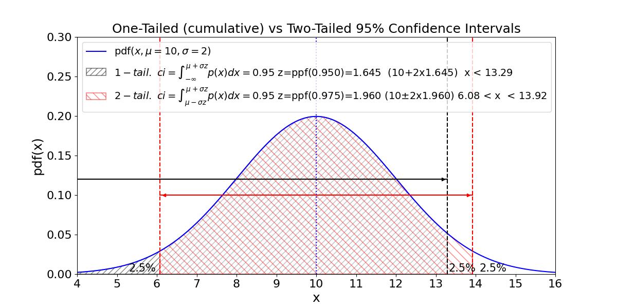
Figure N6 show Python code
  import numpy as np
  import matplotlib.pyplot as plt
  import scipy.stats as stats
  # GLOBAL VARIABLES
  adjst = 0.1  # Adjust arrow heads position
  m = 10
  s = 2
  z_ctr = stats.norm.ppf(0.975)  # 95% CI (2-tailed)
  z_cml = stats.norm.ppf(0.950)  # 95% CI (1-tailed cumulative)

  x1 = m - z_ctr * s
  x2 = m + z_ctr * s
  x3 = m + z_cml * s

  x_ = np.linspace(m - 3 * s, m + 3 * s, 1000)
  y_ = stats.norm.pdf(x_, m, s)

  xh_cml = np.linspace(m - 3 * s, x3, 200)
  yh_cml = np.full_like(xh_cml, 0.12)

  xh_ctr = np.linspace(x1, x2, 200)
  yh_ctr = np.full_like(xh_ctr, 0.1)

  x_fill_cml = np.linspace(m - 3 * s, x3, 200)
  y_fill_cml = stats.norm.pdf(x_fill_cml, m, s)

  x_fill_ctr = np.linspace(x1, x2, 1000)
  y_fill_ctr = stats.norm.pdf(x_fill_ctr, m, s)

  # PLOTS
  fig, ax = plt.subplots(figsize=(12, 6))
  ax.plot(x_, y_, label=r"pdf$(x,\mu=10,\sigma=2)$", color='blue')

  ax.axvline(x1, color='red', linestyle='--')
  ax.axvline(x2, color='red', linestyle='--')
  ax.axvline(x3, color='black', linestyle='--')
  ax.axvline(m, color='blue', linestyle=':')

  ax.plot(xh_cml, yh_cml, color='black')
  ax.plot(x3 - adjst, 0.12, marker='>', markersize=5, color='black')
  ax.plot(x1 + adjst, 0.1, marker='<', markersize=5, color='red')
  ax.plot(x2 - adjst, 0.1, marker='>', markersize=5, color='red')
  ax.plot(xh_ctr, yh_ctr, color='red')

  ax.fill_between(x_fill_cml, y_fill_cml, hatch='///', alpha=0.5,
                  facecolor='white', edgecolor='black', linewidth=1.2,
                  label=r'$1-tail. \ ci=\int_{-\infty}^{\mu+\sigma z}p(x)dx=0.95$'
                  + f' z=ppf(0.950)={z_cml:.3f}  ({m}+{s}x{z_cml:.3f})  x < {x3:.2f}')

  ax.fill_between(x_fill_ctr, y_fill_ctr, hatch='\\\\', alpha=0.5,
                  facecolor='white', edgecolor='red', linewidth=1.2,
                  label=r'$2-tail. \ ci=\int_{\mu-\sigma z}^{\mu+\sigma z}p(x)dx=0.95$'
                  + f' z=ppf(0.975)={z_ctr:.3f} ({m}'+r'$\pm$'+f'{s}x{z_ctr:.3f}) {x1:.2f}
                  < x  < {x2:.2f}')

  # AXES AND GRID
  ax.set_ylim(bottom=0, top=0.3)
  ax.set_xlim(left=m - 3 * s, right=m + 3 * s)

  # TITLE, LABELS, AND ANNOTATIONS
  ax.set_title('One-Tailed (cumulative) vs Two-Tailed 95% Confidence Intervals', fontsize=18)
  ax.set_xlabel('x', fontsize=18)
  ax.set_xticks(range(4,17))
  ax.set_ylabel('pdf(x)', fontsize=18)
  ax.tick_params(axis='both', which='major', labelsize=16)

  # Manually adjust text positions
  ax.text(5.3, 0.003, '2.5%', fontsize=15, color='black')
  ax.text(x3 + 0.03, 0.003, '2.5%', fontsize=15, color='black')
  ax.text(14.1, 0.003, '2.5%', fontsize=15, color='black')

  ax.legend(loc="upper left", fontsize=14)

  # Show plot
  plt.show()
The Gauss Error Function CDF vs ERF
The The Gauss Error Function \(\operatorname{erf}(x)\) is found in Excel, Google Sheets, Python, and on many scientific calculators. However, be very careful if you decide to use it because it is not the same as the cumulative density function (CDF). $$\operatorname{erf}(z) = \frac{2}{\sqrt{\pi}}\int_0^z e^{-t^2} dt, \quad \Phi(z) = \frac{1}{\sqrt{2\pi}} \int_{-\infty}^{z} e^{-\frac{1}{2} t^2} dt$$ $$\text{ERF(z) versus CDF(z)}$$ The two functions are related as follows:
\( \Phi(y) = \frac{1}{2} \left(1 + \operatorname{erf} \left(\frac{y}{\sqrt{2}}\right) \right) \) proofWe are going to use the following identities in this proof:
- \(\operatorname{erf}(z) = \frac{2}{\sqrt{\pi}}\int_0^z e^{-t^2} dt\)
- \(\Phi(z) = \frac{1}{\sqrt{2\pi}} \int_{-\infty}^{z} e^{-\frac{1}{2} t^2} dt\)
- \(\int_{-\infty}^{+\infty} e^{-u^2} \, du = \sqrt{\pi}\), proof:
- \(\text{The total area under the curve of the normal distribution is 1:} \quad \int_{-\infty}^{+\infty}\frac{1}{\sigma\sqrt{2\pi}}e^{-\frac{1}{2}(\frac{x-\mu}{\sigma})^2} \, dx =1\)
- \(\text{Substituting } u=\frac{x-\mu}{\sqrt{2}\sigma} \Rightarrow dx = \sqrt{2}\sigma \, du\)
- \(\int_{-\infty}^{+\infty}\frac{1}{\sqrt{\pi}}e^{-u^2}du=1 \Rightarrow \int_{-\infty}^{+\infty}e^{-u^2}du =\sqrt{\pi}\)
- \(t = \sqrt{2}y \Rightarrow t^2 = 2y^2 \Rightarrow dt=\sqrt{2}dy\)
- \(\text{Due to the symmetry in Equation 3:} \quad \int_{-\infty}^{0}e^{-u^2}du =\frac{\sqrt{\pi}}{2}\)
Substituting \( t \) in Equation 2 using the equalities in step 4: \[ \Phi(z) = \frac{1}{\sqrt{2\pi}} \int_{-\infty}^{\frac{x}{\sqrt{2}}} e^{-y^2}\sqrt{2} \, dy = \frac{1}{\sqrt{\pi}} \int_{-\infty}^{\frac{x}{\sqrt{2}}} e^{-y^2} \, dy \] Splitting the integral: \[ \frac{1}{\sqrt{\pi}} \int_{-\infty}^{\frac{x}{\sqrt{2}}} e^{-y^2} \, dy = \frac{1}{\sqrt{\pi}} \left( \int_{-\infty}^{0} e^{-y^2} \, dy + \int_{0}^{\frac{x}{\sqrt{2}}} e^{-y^2} \, dy \right) \] Using equalities 1 and 5: \[ \Phi(x) = \frac{1}{\sqrt{\pi}} \left(\frac{\sqrt{\pi}}{2} + \frac{\sqrt{\pi}}{2} \operatorname{erf} \left(\frac{x}{\sqrt{2}} \right) \right) = \frac{1}{2} \left(1 + \operatorname{erf} \left(\frac{x}{\sqrt{2}} \right) \right) \] End of proof.
Using the Python cdf function (for the normal distribution): ci = stats.norm.cdf(1) yields ci=0.8413447460685429
Using the Excel erf function: =0.5*(1+ERF(1/SQRT(2))) results in: 0.841344746