Definition and equation derivation

The Poisson distribution is a special case of the binomial distribution when $n \to \infty \ and \ p \to 0$. It is used for predicting the number of independent events k that occur rarely but at a known constant rate $n \lambda$, in a fixed interval of time or space.

The Poisson Distribution: $\bbox[bisque]{P(X = k)= \frac{\lambda^k e^{-\lambda}}{k!} \ k = 0, 1, 2, ...} \ $ derivation

We want to show that the binomial distribution equation becomes the Poisson distribution equation when p is very small and n is very large.

We need to understand a couple of approximations:

for n large and k small: $\frac{n!}{(n-k)!} \approx n^k$

$\frac{n!}{(n-k)!} = \frac{n(n-1)(n-2)...(2)(1)}{(n-k)(n-k-1)(n-k-2)...(2)(1)}=$
$n(n-1)(n-2)...(n-k+1) \leftarrow \text{these are the first k terms of n!}$
if k is small and n is large, the first k terms approximate $n^k$

check: suppose n = 100 and k = 3
then $\frac{n!}{(n-k)!} = 100 \times 99 \times 98 = 970,200 \approx 97 \% \ of \ n^k = 100^3 = 10^6$

for n large and p small: $(1-p)^{n-k} \approx e^{-p(n-k)}$

Taylor series: $f(x) = \sum_\limits{n=0}^{\infty}f^n(a)\frac{(x-a)^n}{n!}, \ f^n \text{ is the }n^{th} \text{ derivative of f}$
First 5 terms of f(x) = ln(1-x) at x = 0:

$ln(1-0)\frac{(x-0)^0}{0!} -(1-0)^{-1} \frac{(x-0)^1}{1!}-(1-0)^{-2} \frac{(x-0)^2}{2!}- $
$2(1-0)^{-3} \frac{(x-0)^3}{3!}-3\times 2(1-0)^{-4} \frac{(x-0)^4}{4!}$

which simplifies to: $ln(1-x) = -x-\frac{x^2}{2}-\frac{x^3}{3}-\frac{x^4}{4}-...$
furthermore for a small x: ln(1-x) = -x.
- check: $ln(1-0.01)\approx 0.01$ the actual value is: -0.010050
$\therefore ln((1-p)^{n-k}) = (n-k)ln(1-p) \approx -p(n-k)$
and $(1-p)^{n-k} \approx e^{-p(n-k)}$ as we wanted to demonstrate

Now start with the binomial distribution equation $$ P(X = k) = \frac{n!}{k!(n - k)!} p^k (1 - p)^{n - k} $$ Substitute in the two approximations demonstrated above: $$ P(X = k) \approx \frac{n!}{k!} p^ke^{-p(n - k)} $$ $ \lambda = np $, thus: $$ P(X = k) \approx \frac{n^k}{k!} \left(\frac{\lambda}{n}\right)^k e^{-\frac{\lambda(n - k)}{n}} $$ $$ P(X = k) \approx \frac{\lambda^k}{k!} \frac{n^k}{n^k} e^{-\lambda + \frac{k \lambda}{n}} $$ As $ n \to \infty $, the term $ \frac{k \lambda}{n} $ approaches 0, so the expression becomes: $$ P(X = k) \approx \frac{\lambda^k}{k!} e^{-\lambda} $$

X: Poisson random variable, k: the number of events

Mean: $\mathbb{E}[X] = \lambda $
Variance: $Var(X) = \lambda $
Standard Deviation: $\sigma \text{_X} = \sqrt{\lambda}$
Coefficient of Variation: $CV = \frac{\sigma \text{_X}}{\mathbb{E}[X]} = \frac{1}{\sqrt{\lambda}}$
The CV is a measure of relative variability. It decreases as $\lambda$ increases.
Here is why in the Poisson distribution $mean = Var = \lambda$: recall that for the binomial distribution $\sigma^2=npq = np(1-p)$. But when p is small $1-p \approx 1$; thus, $\sigma^2 \approx np = \lambda$.

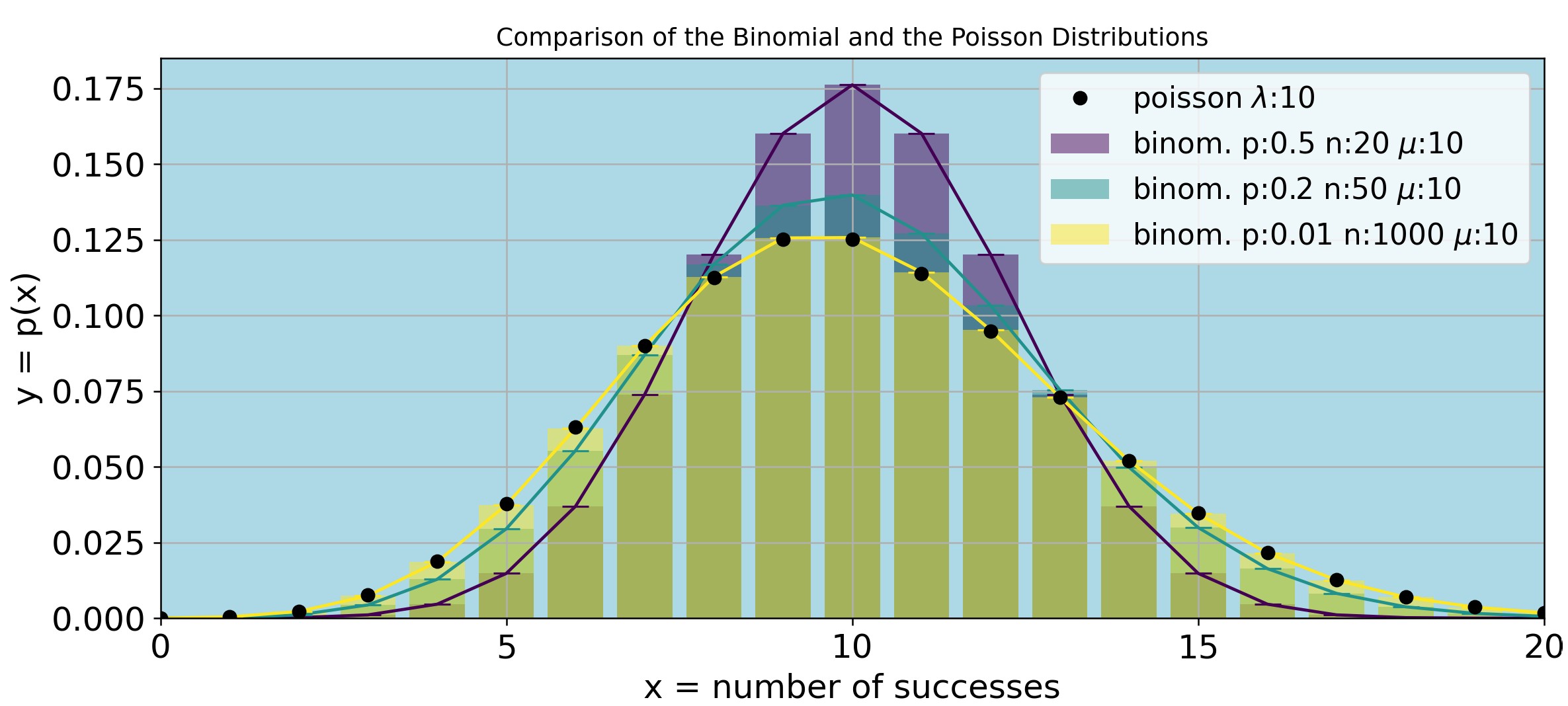
Figure P1 shows that as n gets larger and p gets smaller the Normal and the Poisson distributions superimpose. The Python code for Figure P1 and the derivation of the Poisson distribution equation are respectively shown in the expandable sections below (click the arrows to expand).

Figure P1 show Python code


import numpy as np
import matplotlib.pyplot as plt
from scipy.stats import binom, poisson

# Define the parameters n,p
params = [[20, 0.5], [50, 0.2], [1000, 0.01]]
lmbd = 10
# Create a color map
colors = plt.cm.viridis(np.linspace(0, 1, len(params)))

# Plot the binomial distributions
fig, ax = plt.subplots(figsize=(12,5))
ax.set_facecolor('lightblue')
for i, (n, p) in enumerate(params):
    x = np.arange(0, 25, 1)
    bino_pmf = binom.pmf(x, n, p)
    ax.bar(x, bino_pmf, alpha=0.5, color=colors[i], label=f"binom. p:{p} n:{n} " + r"$\mu$" + f":{n*p:.0f}")
    ax.plot(x, bino_pmf, marker='_', markersize= 13, linestyle='-', color=colors[i])

  # Plot the Poisson distribution
  x = np.arange(0, 25, 1)
  pois_pmf = poisson.pmf(x, lmbd)
  ax.plot(x, pois_pmf, "o", color='black', label=f"poisson " + r"$\lambda$" + f":{lmbd}")

  # Add labels and title
  ax.set_xlabel('x = number of successes',fontsize=16)
  ax.set_xlim(left=0, right=20)
  ax.set_ylabel('y = p(x)', fontsize=16)
  ax.set_title('Comparison of the Binomial and the Poisson Distributions')
  ax.set_xticks([0,5,10,15,20])
  ax.tick_params(axis='x', labelsize=16)
  ax.tick_params(axis='y', labelsize=16)
  ax.legend(fontsize=14)
  ax.grid(True)
  plt.show()

Shape of the Poisson Distribution for Different Expected Values

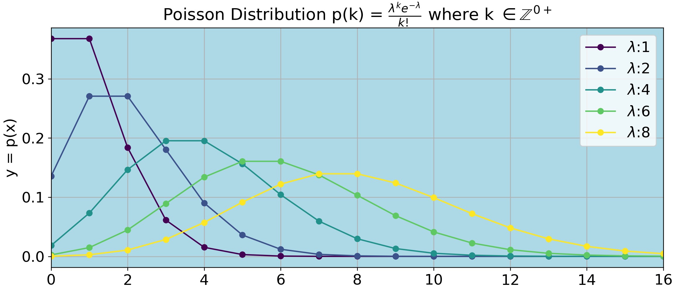
Figure P2 shows the shape of the Poisson distribution for $\lambda = 1 \rightarrow 8$. Note that $\lambda$ (the expected value) is a real positive number, but k (the number of observations, corresponding to the number of successes in the binomial distribution) can only be 0 or an integer. Therefore the lines on Figure P2 are just for guidance, they do not represent continuous values for p(k).

For example, say you expect to see a mutation that will restore bacterial growth at a rate of 4 mutations per 10⁸ bacteria. That is, if you plate 10⁸ bacteria you expect to see 4 colonies on the plate on the next day. Thus, $\lambda=4$; however, you do not necessarily see exactly 4 colonies the next day. If you plate 10⁸ bacteria on each of 10 plates you should see that the number of colonies k on each plate will follow the distribution shown on the dark green curve of Figure P2.

Figure P2 show Python code


          import numpy as np
          import matplotlib.pyplot as plt
          from scipy.stats import binom, poisson
          
          # Create a color map
          colors = plt.cm.viridis(np.linspace(0, 1, 5))
          
          # Plot the binomial distributions
          fig, ax = plt.subplots(figsize=(12,5))
          ax.set_facecolor('lightblue')
          lbnd_values = [1,2,4,6,8]
          # Plot the Poisson distribution
          x = np.arange(0, 17, 1)
          for i, lmbd in enumerate(lbnd_values):
              pois_pmf = poisson.pmf(x, lmbd)
              ax.plot(x, pois_pmf, "o", color=colors[i], linestyle='-',label=fr'$\lambda$:{lmbd}')
          
          # Add labels and title
          ax.set_xlabel(f'k',fontsize=16)
          ax.set_xlim(left=0, right=16)
          ax.set_ylabel(f'y = p(x)', fontsize=16)
          ax.set_title(r'Poisson Distribution p(k) = 
          $\frac{\lambda^k e^{-\lambda}}{k!}$ where k $\in \mathbb{Z}^{0+}$', fontsize=18)
          ax.legend(fontsize=16)
          ax.set_xticks(np.arange(min(x), max(x)+1, 2))
          ax.tick_params(axis='x', labelsize=16)
          ax.tick_params(axis='y', labelsize=16)
          ax.grid(True)
          plt.show()

Examples and Applications

Confidence in detecting a rare event in a given interval

A study by Kim et al. (1996) examined the probability of capturing a specific region of the human genome in a genomic library. The authors reported:

“We have constructed an arrayed human genomic BAC library with approximately 4x coverage, represented by 96,000 BAC clones with an average insert size of nearly 140 kb. … More than 92% of the probes used to screen the library identified one or more hits. This is close to the 98% frequency predicted by a Poisson distribution for recovery of any marker from a 4x library.”

Let us check their numbers

The total base pairs covered by the library:
$ 96,000 \text{ BAC clones} \times \frac{140,000 \text{ bp}}{\text{BAC clone}} = 1.344 \times 10^{10} \text{ bp} $
The human genome is approximately $ 3 \times 10^9 $ base pairs. The library coverage is therefore:
$ \frac{1.344 \times 10^{10} \text{ bp}}{3 \times 10^9 \text{ bp/hu genome}} = 4.48\times hu \ genome $
This confirms that the library provides approximately 4.48x coverage, close to the reported 4x.

The probability of not capturing the marker (i.e., it appears 0 times) is:
$ P(k = 0 \mid \lambda = 4) = \frac{\lambda^k e^{-\lambda}}{k!} = \frac{4^0 e^{-4}}{0!} = e^{-4} = 0.01832 $
The probability of detecting the marker at least once is:
$ 1 - P(k = 0) = 1 - 0.01832 = 0.982 $
This confirms Kim et al.'s statement that the expected probability of recovering a marker from a 4× library is about 98%.

How many clones should they screen for a 99% confidence of detecting a particular DNA region?

The library has 4x genome coverage and contains 96,000 clones.
On average, a given DNA region should be present in:
$ \frac{96,000}{4} = 24,000 $ clones.
To find the number of clones needed for 99% confidence:
- We solve for $ \lambda $ in:
  $ P(k = 0 \mid \lambda) = \frac{\lambda^k e^{-\lambda}}{k!} = e^{-\lambda} = 0.01 $
- Taking the natural logarithm:
  $ \lambda = -\ln(0.01) \approx 4.6 $
- Since the region appears, on average, once per 24,000 clones, we must screen:
  $ 4.6 \times 24,000 = 110,400 $ clones.
Thus, screening 110,400 clones ensures a 99% chance of detecting the region.

1. Modeling Disease Incidence Rates

Consider a scenario where a rare disease occurs at an average rate of 2 cases per 100,000 people annually. The probability of observing $ k $ cases in a year can be modeled using the Poisson distribution with $ \lambda = 2 $.

2. Counting Adverse Events in Clinical Trials

Example: If patients experience a side effect at a rate of 1 per 100 patient-days, the probability of observing a certain number of side effects in 500 patient-days can be calculated using $ \lambda = 5 $.

The Chi-Square Distribution in the Context of the Poisson Distribution

The chi-square distribution is often used in conjunction with the Poisson distribution particularly in hypothesis testing and constructing confidence intervals for Poisson rates.

1. Goodness-of-Fit Tests

The chi-square test assesses how well the observed data fit the expected frequencies under the Poisson model:

Example: Suppose we have observed counts of infections over several intervals. We can use the chi-square test to determine if the data follow a Poisson distribution.

The test statistic is calculated as:

$$ \chi^2 = \sum_{i=1}^k \frac{(O_i - E_i)^2}{E_i} $$

$ O_i $: Observed frequency for interval $ i $
$ E_i $: Expected frequency under the Poisson model for interval $ i $

2. Confidence Intervals for Poisson Rates

When estimating the confidence interval for a Poisson rate, the chi-square distribution provides critical values:

$$ \text{Confidence Interval for } \lambda: \left( \frac{1}{2}\chi^2_{\alpha/2,2k}, \frac{1}{2}\chi^2_{1-\alpha/2,2(k+1)} \right) $$

$ k $: Observed number of events
$ \chi^2_{\alpha, \nu} $: The chi-square critical value with significance level $ \alpha $ and degrees of freedom $ \nu $

3. Poisson Regression and Deviance Testing

In Poisson regression models, which are used to model count data, the deviance (a measure of goodness-of-fit) follows a chi-square distribution. This allows for hypothesis testing about the predictors in the model. ......

•^⅄ AbAETERNUM antibodies forever

CHAPTER 5: THE POISSON DISTRIBUTION