In this chapter we discuss general concepts and equations. When these are applied to different distributions they give rise to other equations that are used in practice, as discussed in the chapters focusing on the specific distributions.
Random Experiments
A random experiment can yield different results despite being performed under the same conditions. For example, each tossing of a coin can have two possible results: heads or tails. Another example is the measurement of the absorbance of a solution, which, if done in triplicate under the same conditions, can have different values albeit close to some expected average.
Sample Space
A sample space is the set of all possible outcomes of a random experiment. For example if we toss a die just once the sample space has 6 possible sample points: {1,2,3,4,5,6}. But if we toss it twice the sample space now has 36 points {(1,1),(1,2),(1,3),...(6,6)}
Random Variable
A random variable, usually denoted by a capital X or by a capital Y, is the numerical outcome of a random experiment. Random variables can be discrete or continuous. For example, if we count the number of heads while tossing a coin 10 times, and we get 4 heads, then X = 4, and this is a discrete random variable because X is always either 0 or an integer. If we measure the absorbance of a solution and obtain 1.384, then X = 1.384 and that is a continuous random variable because its sample space consists of a continuous range of real numbers.
Probability Mass Function (PMF), Probability Density Function (PDF), and Cumulative Distribution Function (CDF)
A function is a probability function or probability distribution if it satisfies the following criteria:
- It yields the probability of a random variable \( X \) being equal to a specific value. Caution: this criterion is interpreted differently for discrete versus continuous variables (see below).
- \( 0 \le f(x) \le 1 \). The probability cannot be negative or larger than 1.
- The total probability across all possible outcomes is 1.
For a discrete random variable \( X \), the probability function is called a probability mass function (PMF). It gives the probability that \( X \) takes on the value \( x \): \( P(X = x) = p(x) \).
For a continuous random variable, the probability function is called a probability density function (PDF). In this case, \( P(X = x) = 0 \) for any real number \( x \), because the variable can take infinitely many values even within a very small interval (e.g., from 1.000 to 1.001). Therefore, the PDF does not give the probability at a point, but rather a density. To compute the probability over an interval \( [a, b] \), we integrate the PDF: \( P(a \leq X \leq b) = \int_a^b f(x) \, dx \)
The total probability for a discrete variable is: \( \sum_x p(x) = 1 \). For a continuous variable, it is: \( \int_{-\infty}^{+\infty} f(x) \, dx = 1 \). This represents the total area under the curve. If the range of a continuous variable \( X \) is restricted to \( a \le x \le b \), then:
\( \int_{-\infty}^{a} f(x) \, dx = 0, \quad \int_a^b f(x) \, dx = 1, \quad \int_b^{+\infty} f(x) \, dx = 0 \)
A Cumulative Distribution Function (CDF) gives the probability that a random variable \( X \) is less than or equal to a given value \( x \).
For a discrete variable: \( CDF(x) = \sum\limits_{x_i = x_{\text{min}}}^{x} p(x_i) \)
For a continuous variable: \( CDF(x) = \int_{-\infty}^x f(x) \, dx \)
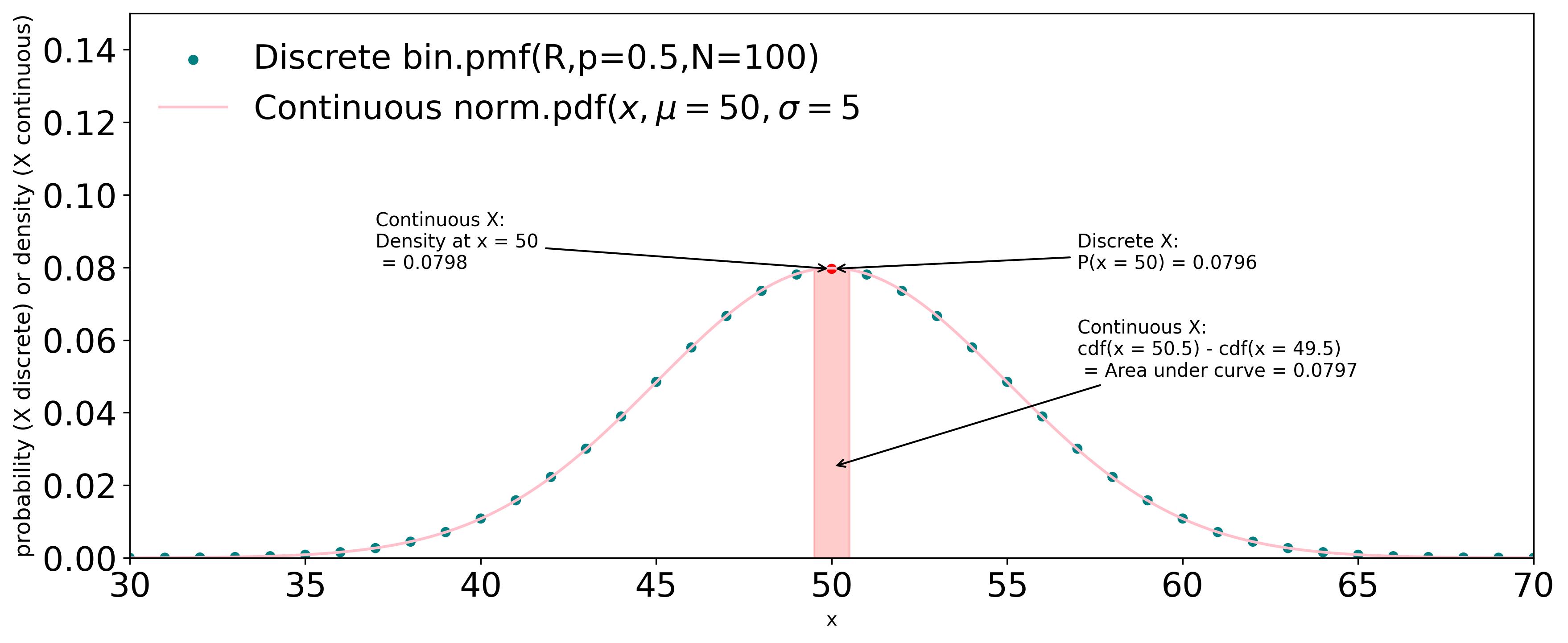 Figure G1 shows a plot of a binomial distribution PMF for N = 100 and p(x) = 0.5,
superimposed with a normal distribution PDF with the same mean and standard deviation
as the PMF:
$$\mu = Np = 50, \ \sigma=\sqrt{Npq} = 5, \ where \ q = 1 - p$$
One can use the same scale on the y-axis
but the numbers mean different things: probability for
PMF and density for the PDF. To calculate the probability of the continuous variable between
x = 49.5 and x = 50.5, we subtracted the CDF(50.5) from CDF(49.5).
show Python code
Figure G1 shows a plot of a binomial distribution PMF for N = 100 and p(x) = 0.5,
superimposed with a normal distribution PDF with the same mean and standard deviation
as the PMF:
$$\mu = Np = 50, \ \sigma=\sqrt{Npq} = 5, \ where \ q = 1 - p$$
One can use the same scale on the y-axis
but the numbers mean different things: probability for
PMF and density for the PDF. To calculate the probability of the continuous variable between
x = 49.5 and x = 50.5, we subtracted the CDF(50.5) from CDF(49.5).
show Python code
Python code for Figure G1
  import numpy as np
  import matplotlib.pyplot as plt
  import math
  from scipy.stats import norm
  from scipy.stats import binom

  # DISTRIBUTION PARAMETERS
  N = 100
  p = 1/2 # binomial probability (e.g. coin toss h vs t)
  mu,v,sk,k = binom.stats(N,p,moments="m,v,s,k")
  s = math.sqrt(v) # standard deviation
  R_ = list(range(N+1)) # [0, 1, 2, ... 100] 101 possible values for binomial

  # X AND Y VALUES AND RANGES TO BE PLOTTED
  P_ = binom.pmf(R_,N,p)
  xmin = 30
  xmax = 70
  x_ = np.linspace(xmin,xmax,300)
  y_ = norm.pdf(x_,mu,s)
  Pof50 = binom.pmf(50,N,p)
  fOf50 = norm.pdf(50,mu,s)
  cdfAround50 = norm.cdf(50.5,mu,s) - norm.cdf(49.5,mu,s)
  x_fill = np.linspace(49.5,50.5,100)
  y_fill = norm.pdf(x_fill,mu,s)

  #FIGURE PARAMETERS
  fig, ax = plt.subplots(figsize=(12,5))
  binMrkrColors = ['teal']*len(R_)
  binMrkrColors[50] = 'red'
  ax.tick_params(axis='both', which='major', labelsize=18)
  ax.set_title(r'Discrete Binomial (N = 100, p = 0.5) versus Continuous Normal $(\mu = 50 \ \sigma = 5)$ Distributions',
                fontsize=14)

  #ANNOTATIONS WITH ARROWS
  ax.annotate(
      f'Discrete X:\nP(x = 50) = {Pof50:.4f}',
      xy=(50,Pof50),
      xytext=(57,Pof50),
      arrowprops=dict(facecolor='black', arrowstyle='->'),
      fontsize=14
  )
  ax.annotate(
      f'Continuous X:\nDensity at x = 50\n = {fOf50:.4f}',
      xy=(50,Pof50),
      xytext=(37,Pof50),
      arrowprops=dict(facecolor='black', arrowstyle='->'),
      fontsize=14
  )
  ax.annotate(
      f'Continuous X:\ncdf(x = 50.5) - cdf(x = 49.5)\n = Area under curve = {cdfAround50:.4f}',
      xy=(50,0.025),
      xytext=(57,0.05),
      arrowprops=dict(facecolor='black', arrowstyle='->'),
      fontsize=14
  )

  # AXES
  ax.set_xlabel(f'x',fontsize=14)
  ax.set_ylabel(r'PMF (discrete) or PDF (continuous)',fontsize=14)
  ax.set_xlim(left=30, right=70)
  ax.set_ylim(bottom=0, top=0.15)

  # PLOT
  ax.scatter(R_, P_, marker="o",  s = 20, color=binMrkrColors,
              label=r'binom.pmf(R,p=0.5,N=100)')
  ax.plot(x_, y_, linestyle="-", marker="none", color='pink',
            label=r'norm.pdf($x,\mu=50,\sigma=5$)')
  ax.fill_between(x_fill,y_fill,color='red', alpha=0.2)
  ax.legend(loc="upper left", frameon=False,fontsize=14)


  #ADJUST LAYOUT AND SAVE FIGURE THEN SHOW IT
  plt.tight_layout()
  plt.savefig("AAA.jpeg", dpi=300, bbox_inches='tight')
  plt.show()
Mathematical Expectation, Mean, Median, Mode, and Percentiles
The mathematical expectation, is an operator written as \(\mathbb{E}\)[ ] or as E[ ], which is used to define several "statistics" such as the mean, the variance, the skewness and the kurtosis, as well as functions such as the moment generating function.
The expectation of X is the mean of its distribution.
For a discrete random variable with a probability mass function f(x), it is the weighted average of all possible values of X, where each value is weighted by its corresponding frequency: $$\mathbb{E}[X] = \sum\limits_{i=1}^{n}x_if(x_i) = \mu$$ For a continuous random variable with a probability density function f(x): $$\mathbb{E}[X] = \int_{-\infty}^{+\infty}xf(x)dx = \mu$$
Properties of \(\mathbb{E}\)[ ]
- \(\mathbb{E}[cX] = c\mathbb{E}[X] \ \) we can pull a constant out of the expectation
- it follows from above that \(\mathbb{E}[c] = c \ \) the expectation of a constant is the constant
- \(\mathbb{E}[X + Y] = \mathbb{E}[X] + \mathbb{E}[Y]\ \ \) the expectation of a sum is the sum of the expectations
- \(\mathbb{E}[XY] = \mathbb{E}[X]\mathbb{E}[Y]\ \ \) for INDEPENDENT X Y variables, the expectation of a product is the product of the expectations
The mode is the value of the random variable that has the highest occurrence probability. For a continuous probability function (PDF) it is the value of x corresponding to the maximum density.
The median, and the percentiles or quartiles are calculated differently, depending on whether we are referring to datasets or to probability distributions. This is best explained examples. Take the following dataset with 9 values. Quartiles are either individual data points or the average of two adjacent points (shown in bold).
Dataset = [0.01, 0.02, 0.03, 0.04, 0.05, 0.06, 0.07, 0.50, 0.22]
| 1st | 2nd = Median | 3rd | |
|---|---|---|---|
| Quartiles | \(\frac{0.02+0.03}{2}=0.025\) | 0.05 | \(\frac{0.07+0.50}{2}=0.285\) |
Of course, there is little or nothing to reveal by dividing a dataset of 9 data points into quartiles. Quartiles or percentiles are especially useful when you have large datasets, such the weights of newborns in a certain year and region of the country. But this small dataset is useful to help understand the calculation procedure, which is as follows:
- First the dataset must be sorted in ascending order.
- The median is the datapoint in the middle of the set. If the set has an even number of elements, then the median is the average of the two middle elements
- The quartiles are respectively the datapoints or the average of 2 datapoints that separate the first quarter, the first half, and the first 3/4 of the data from the rest of the data. The second quartile is the same as the median.
- You can extend the process to deciles (10% groups) or percentiles by dividing the data by any number, provided you have enough datapoints.
Let us now calculate the median and the quartiles for a discrete probability distribution. Let the following array be the complete set of probabilities of a discrete random variable. The probabilities are all non-negative and add up to 1, as required.
X = [1, 2, 3, 4, 5, 6, 7, 8, 9], P(X) = [0.01, 0.02, 0.03, 0.04, 0.05, 0.06, 0.07, 0.50, 0.22]
This means that, for example, P(X = 8) = 0.5.
| 1st | 2nd = median | 3rd | |
|---|---|---|---|
| Quartiles | \(x_j | \sum\limits_{i=1}^{j}P(x_i) \ge 0.25 \rightarrow x = 7\) | \(x_j | \sum\limits_{i=1}^{j}P(x_i) \ge 0.50 \rightarrow x = 8\) | \(x_j | \sum\limits_{i=1}^{j}P(x_i) \ge 0.75 \rightarrow x = 8\) |
| PMF(xj) | 0.07 | 0.50 | 0.50 |
| CDF(xj) | 0.28 | 0.78 | 0.78 |
In this case, the values of X must be sorted in ascending order, and the corresponding probabilities must remain aligned. Then, the CDF is computed cumulatively until each quartile threshold is met.
Finally, in the case of a continuous random variable the median is simply the x value for which the cumulative probability distribution is 0.5. The same principle applies for calculating quartiles, deciles or percentiles. $$\int_{-\infty}^xf(x)\,dx = 0.5$$ For example $$f(x) = x^2\Big|_0^{\sqrt[3]{3}}$$ is a PDF because its total probability within its boundaries is 1. $$\int_0^{\sqrt[3]{3}}x^2\,dx = \frac{1}{3}x^3 \Big|_0^{\sqrt[3]{3}} = 1$$ Its median is: $$\sqrt[3]{\frac{3}{2}} \approx 1.34 \quad \text{because} \quad \int_0^{\sqrt[3]{\frac{3}{2}}} x^2 \, dx = \frac{1}{3} x^3 \Big|_0^{\sqrt[3]{3/2}} = 0.5$$ Its mode is: \(\sqrt[3]{3}\) - the value of x where the PDF f(x) = x2 reaches its maximum within the support. (Note: in statistics support is the set of values that the random variable can take and for which the PDF or PMF is positive).
Its mean is: $$\int_0^{\sqrt[3]{3}}xx^2\,dx = \frac{1}{4}x^4|_0^{\sqrt[3]{3}} = \frac{1}{4}3^{\frac{4}{3}} \simeq 1.08 $$
Interactive Plot With Quartiles: Binomial PMF vs Normal PDF
Figure G2 (Interactive): Superimposed plots or the binomial and normal distributions. Play with the sliders to change binomial N and p (probability of success). Refreshing the page resets these parameters to N = 22 and p = 0.20. The statistical parameters mean (\(\mu\)), and standard deviation (\(\sigma\)) are the same for both distributions. The mode, skewness, and kurtosis apply only to the binomial distribution because in the normal distribution the mode, the median and the mean are the same (\(\mu\)) and the skewness and kurtosis are always 0 and 3, respectively. The first, second (median) and third quartiles, are indicated by colored (green, red, green) bars for the binomial distribution or red dots for the normal distribution.
Variance and Standard Deviation
The variance is a measure of the spread of the distribution and of the
variability of the data. The standard deviation
is the square root of the variance. In a normal distribution, the standard
deviation corresponds to the distance from the mean to the inflection
point of the curve.
$$Var(X) = \sigma^2 = \mathbb{E}[(X - \mu)^2] = \mathbb{E}[(X - \mathbb{E}[X])^2]$$
The standard deviation is \(\sigma\).
For a continuous distribution such as the normal distribution,
$$\sigma^2 = \int_{-\infty}^{+\infty} (x - \mu)^2 f(x) dx$$
Important variance equalities
- \(Var(X) = \mathbb{E}[X^2] - \mathbb{E}[X]^2\ \)
proof
- \(Var(X) = \mathbb{E}[(X - \mathbb{E}[X])^2]\)=
- \(\mathbb{E}[(X^2 - 2X\mathbb{E}[X] + \mathbb{E}[X]^2)\)=
- \(\mathbb{E}[X^2] - 2\mathbb{E}[X\mathbb{E}[X] + \mathbb{E}[\mathbb{E}[X]^2]\)=
- \(\mathbb{E}[X^2] - 2\mathbb{E}[X]\mathbb{E}[X] + \mathbb{E}[X]^2\)=
- \(\mathbb{E}[X^2] - 2 (\mathbb{E}[X])^2 + \mathbb{E}[X]^2 = \)
- \(\mathbb{E}[X^2] - \mathbb{E}[X]^2\)
- \(Var(cX) = c^2 Var(X)\ \) you can pull a constant out of the Var but you have to square it
proof
- \(Var(cX) = \mathbb{E}[(cX - \mathbb{E}[cX])^2]=\)
- \(\mathbb{E}[c^2X^2 - 2c^2X\mathbb{E}[X] + c^2\mathbb{E}[X]^2]=\)
- \(c^2\mathbb{E}[X^2 - 2X\mathbb{E}[X] + \mathbb{E}[X]^2]=\)
- \(c^2\mathbb{E}[(X^2 - \mathbb{E}[X])^2]=\)
- \(c^2Var(X)\)
- Var(X + Y) = Var(X) + Var(Y) + 2Cov(X,Y)
Var(X - Y) = Var(X) + Var(Y) - 2Cov(X,Y) proof- \(Var(X+Y)= \mathbb{E}[(X+Y-\mathbb{E}[X+Y])^2=\mathbb{E}[(X+Y-\mathbb{E}[X]-\mathbb{E}[ Y])^2=\)
- \(\mathbb{E}[((X-\mathbb{E}[X])+(Y-\mathbb{E}[ Y]))^2=\)
- \(\mathbb{E}[(X-\mathbb{E}[X])^2 + 2(X-\mathbb{E}[X])(Y-\mathbb{E}[Y]) + (Y-\mathbb{E}[Y])^2]=\)
- \(\mathbb{E}[(X-\mathbb{E}[X])^2] + 2\mathbb{E}[(X-\mathbb{E}[X])(Y-\mathbb{E}[Y])] + \mathbb{E}[(Y-\mathbb{E}[Y])^2]=\)
- \(Var(X) + 2Cov(X,Y) + Var(Y)\)
- for Var(X - Y) the middle term in 5 would be \(- 2Cov(X,Y)\)
- Corolary: if X and Y are uncorrelated, that is, independent random variables, then Cov(X,Y) = 0; therefore:
- Var(X + Y) = Var(X) + Var(Y) for independent X,Y
- Var(X - Y) = Var(X) + Var(Y) for independent X,Y
- Var(\(\sum X_i\)) = \(\sum Var(X_i)\) this is an extension of 4.a
- \(Var(\bar{X})=\frac{\sigma^2}{n}\)
proof
- \(Var(\bar{X}) = Var\left(\frac{1}{n} \sum x_i\right)\)
- \(=\frac{1}{n^2}Var(\sum{x_i})\) using equality 2
- \(=\frac{1}{n^2}\sum{Var(x_i)}\) using equality 5
- \(=\frac{1}{n^2}\sum{\sigma^2}\)
- \(=\frac{n\sigma^2}{n^2} \ because \ \sigma^2 \text{ is a constant}\)
- \(=\frac{\sigma^2}{n}\)
- \(\mathbb{E}[X^2] = \sigma^2 + \mu^2\)
proof
- \(\sigma^2 = \mathbb{E}[(X - \mathbb{E}[X])^2]\)
- \(\sigma^2 = \mathbb{E}[(X - \mu)^2]\)
- \(\sigma^2 = \mathbb{E}[X^2 - 2X\mu + \mu^2]\)
- \(\sigma^2 = \mathbb{E}[X^2] - 2\mu\mathbb{E}[X] + \mu^2\)
- \(\sigma^2 = \mathbb{E}[X^2] - 2\mu^2 + \mu^2\)
- \(\sigma^2 = \mathbb{E}[X^2] - \mu^2\)
- \(\mathbb{E}[X^2] = \sigma^2 + \mu^2\)
- \(\mathbb{E}[{\bar{X}}^2] = \frac{\sigma^2}{n} + \mu^2\)
proof
- Recall equality 1: \(Var(X) = \mathbb{E}[X^2] - \mathbb{E}[X]^2\)
- Therefore: \(Var(\bar{X}) = \mathbb{E}[{\bar{X}}^2] - \mathbb{E}[\bar{X}]^2\)
- \(Var(\bar{X}) = \mathbb{E}[{\bar{X}}^2] - \mu^2\)
- \(\mathbb{E}[{\bar{X}}^2] = Var(\bar{X}) + \mu^2\)
- Apply equality 6: \(\mathbb{E}[{\bar{X}}^2] = \frac{\sigma^2}{n} + \mu^2\)
The Sample Variance Equation
Population Variance: \(\sigma^2=\frac{\sum(x_i - \mu)^2 }{N}\)Sample Variance: \(\bbox[bisque]{s^2=\frac{\sum(x_i - \bar{x})^2 }{n-1}}\) derivation
Which is a better estimator of the true variance:
\(\frac{\sum(x_i-\bar{x})^2}{n} \ or \ \frac{\sum(x_i-\bar{x})^2}{n-1}\)?
Let A be a variable that could take either of the values: A = n or A = n - 1.
- \(\mathbb{E}[\frac{\sum(x_i-\bar{x})^2}{A}]=\)
- \(\frac{1}{A}\mathbb{E}[\sum(x_i-\bar{x})^2]=\)
- \(\frac{1}{A}\mathbb{E}[\sum({x_i}^2-2\bar{x}x_i + \bar{x}^2)]=\)
- \(\frac{1}{A}\mathbb{E}[\sum{{x_i}^2}-2\bar{x}\sum{x_i} + n\bar{x}^2]=\)
- \(\frac{1}{A}\mathbb{E}[\sum{{x_i}^2}-2\bar{x}n\bar{x} + n\bar{x}^2]=\)
- \(\frac{1}{A}\mathbb{E}[\sum{{x_i}^2} - n\bar{x}^2]=\)
- \(\frac{1}{A}(\sum{\mathbb{E}[{x_i}^2]} - n\mathbb{E}[\bar{x}^2])=\)
At this point note the following equalities (see Chapter 1 /Variance ...)
- \( \mathbb{E}[X^2] = \sigma^2 + \mu^2 \)
- \( \mathbb{E}[\bar{X}^2] = \frac{\sigma^2}{n} + \mu^2 \)
- \(\frac{1}{A}(\sum(\sigma^2 + \mu^2) - n(\frac{\sigma^2}{n} + \mu^2))=\)
- \(\frac{1}{A}(n\sigma^2 + n\mu^2 - \sigma^2 - n\mu^2)=\)
- \(\frac{(n-1)\sigma^2}{A}\)
Therefore: \(\mathbb{E}[\frac{\sum(x_i-\bar{x})^2}{A}]=\sigma^2\) only if A = n - 1. Thus, using n - 1 in the denominator makes the sample variance an unbiased estimator of the population variance.
The population variance equation is valid only if we know the entire population's mean - note the denominator of the fraction N. However, we usually work with samples, for which we do not know the true mean. In this case, the denominator of the fraction is n - 1 instead of N. This is to correct for the fact that dividing by N tends to yield an underestimate of the variance. This underestimate arises from the smaller spread of the sample when compared to its true spread. Dividing by n-1 will increase the estimate of the variance. Click "derivation" after the equation to see the math that justifies this correction.
Covariance
Random variables X and Y, with a probability distribution \(f^{}_{X,Y}(x,y)\) can be correlated, meaning
that a change in X is associated with a change in Y and vice-versa.
We can then define their covariance as:
\(Cov(X,Y)=\mathbb{E}[(X-\mathbb{E}[X])(Y-\mathbb{E}[Y])]\)
A positive covariance means that the random variables tend to increase together;
Conversely, a negative variance indicates that the tendency of one variable to increase
correlates with the tendency of the other to decrease.
Important covariance equalities
- \(Cov(X,Y) = \mathbb{E}[XY] - \mathbb{E}[X]\mathbb{E}[Y] = \mathbb{E}[XY]-\mu^{}_{X}\mu^{}_{Y} \)
proof
- \(Cov(X,Y) = \mathbb{E}[(X - \mathbb{E}[X])(Y - \mathbb{E}[Y])]\)
- \(= \mathbb{E}[XY - X\mathbb{E}[Y] - \mathbb{E}[X]Y + \mathbb{E}[X]\mathbb{E}[Y]]\)
- \(= \mathbb{E}[XY] - \mathbb{E}[X]\mathbb{E}[Y] - \mathbb{E}[X]\mathbb{E}[Y] + \mathbb{E}[X]\mathbb{E}[Y]\)
- \(= \mathbb{E}[XY] - \mathbb{E}[X]\mathbb{E}[Y]\)
- \(Cov(X,X) = Var(X)\)
proof
- \(Cov(X,X) = \mathbb{E}[(X - \mathbb{E}[X])(X - \mathbb{E}[X])]\)
- \(= \mathbb{E}[(X - \mathbb{E}[X])^2] = Var(X)\)
- \(Cov(X, c) = 0\) for any constant \(c\)
proof
- \(Cov(X, c) = \mathbb{E}[(X - \mathbb{E}[X])(c - \mathbb{E}[c])]\)
- \(= \mathbb{E}[(X - \mathbb{E}[X])(c - c)] = \mathbb{E}[(X - \mathbb{E}[X]) \cdot 0] = 0\)
- \(Cov(aX, bY) = abCov(X,Y)\). Bilinearity: in contrast with variance which scales with
the square of a constant, covariance scales multiplicatively with constants.
proof
- \(Cov(aX, Y) = \mathbb{E}[(aX - \mathbb{E}[aX])(bY - \mathbb{E}[bY])]\)
- \(= \mathbb{E}[ab(X - \mathbb{E}[X])(Y - \mathbb{E}[Y])]\)
- \(= ab\mathbb{E}[(X - \mathbb{E}[X])(Y - \mathbb{E}[Y])] = abCov(X,Y)\)
- \(Cov(X + Z, Y) = Cov(X, Y) + Cov(Z, Y)\) Additivity of covariance
proof
- \(Cov(X + Z, Y) = \mathbb{E}[(X + Z - \mathbb{E}[X + Z])(Y - \mathbb{E}[Y])]\)
- \(= \mathbb{E}[(X - \mathbb{E}[X] + Z - \mathbb{E}[Z])(Y - \mathbb{E}[Y])]\)
- \(= \mathbb{E}[(X - \mathbb{E}[X])(Y - \mathbb{E}[Y]) + (Z - \mathbb{E}[Z])(Y - \mathbb{E}[Y])]\)
- \(= Cov(X,Y) + Cov(Z,Y)\)
- \(Cov(\sum \limits_{i=1}^{n} a_iY_i,\sum \limits_{j=1}^{n} b_jY_j) =\sum \limits_{i=1}^{n}\sum \limits_{j=1}^{n}a_ib_j Cov(Y_i, Y_j)\)
Double sum for any constants ai and bj
proof
- Apply equality 1: \(Cov(\sum \limits_{i=1}^{n} a_iY_i,\sum \limits_{j=1}^{n} b_jY_j) =\mathbb{E}[(\sum \limits_{i=1}^{n} a_iY_i)(\sum \limits_{j=1}^{n} b_jY_j)] - \mathbb{E}[\sum \limits_{i=1}^{n} a_iY_i]\mathbb{E}[\sum \limits_{j=1}^{n} b_jY_j]\)
-
- Term 1: \(\mathbb{E}[(\sum \limits_{i=1}^{n} a_iY_i)(\sum \limits_{j=1}^{n} b_jY_j)]=\sum \limits_{i=1}^{n}\sum \limits_{j=1}^{n}a_ib_j\mathbb{E}[Y_iY_j]\)
- Term 2: \(\mathbb{E}[\sum \limits_{i=1}^{n} a_iY_i]\mathbb{E}[\sum \limits_{j=1}^{n} b_jY_j]= \sum \limits_{i=1}^{n} a_i\mathbb{E}[Y_i]\sum \limits_{j=1}^{n} b_j\mathbb{E}[Y_j]=\sum \limits_{i=1}^{n}\sum \limits_{j=1}^{n}a_ib_j\mathbb{E}[Y_i]\mathbb{E}[Y_j]\)
- Subtract term 2 from term 1: \(\sum \limits_{i=1}^{n}\sum \limits_{j=1}^{n}a_ib_j(\mathbb{E}[Y_iY_j] - \mathbb{E}[Y_i]\mathbb{E}[Y_j]) \)
- Apply equality 1 again: \(\sum \limits_{i=1}^{n}\sum \limits_{j=1}^{n}a_ib_jCov(Y_i,Y_j)\)
Correlation Coefficient
The correlation coefficient r or "\(\color{red}{\rho}\)" or Pearson's correlation coefficient is a statistical quantification of the strength and direction of the linear relationship between two variables. $$\rho = \frac{cov(X,Y)}{\sigma^{}_{X}\sigma^{}_{Y}}$$ $$\rho_{xy} = \frac{\sum((x_i-\bar{x})(y_i-\bar{y}))}{\sqrt{\sum(x_i-\bar{x})^2}\sqrt{\sum(y_i-\bar{y})^2}}$$ If there is no correlation their covariance is zero, \(Cov(X,Y) = \mathbb{E}[(X-\mathbb{E}[X])(Y-\mathbb{E}[Y])]=0\). In contrast, if there is a perfect correlation, the product of their standard deviations equals the absolute value of the covariance. \(|cov(X,Y)| = \sigma^{}_{X}\sigma^{}_{Y}\). The closer r is to -1 or to 1 the stronger the negative or positive correlation, and the closer the value is to 0 the weaker the correlation.
If X and Y are perfectly correlated, (i.e. Y = aX + b) \(|cov(X,Y)| = \sigma^{}_{X}\sigma^{}_{Y}\) proof- If X and Y are perfectly correlated then, Y = aX + b
- Show that \({\sigma^{}_{Y}}^2 = a^2{\sigma^{}_{X}}^2\)
\(\mathbb{E}[(Y - \mu^{}_{Y})^2] = \mathbb{E}[(aX+b-\mathbb{E}(aX + b))^2]=\)
\(\mathbb{E}[(aX+b-a\mathbb{E}[X]-b)^2]=a^2\mathbb{E}[(X-\mathbb{E}[X])^2]=a^2{\sigma^{}_{X}}^2\)
- The stDevY is thus: \(\sigma^{}_{Y} = |a|\sigma^{}_{X}\)
- Express in terms of the StDevX: \(\sigma^{}_{X} = \frac{\sigma^{}_{Y}}{|a|}\)
- Show that \(cov(X,Y) = a{\sigma^{}_{X}}^2 \)
\(cov(X, Y) = \mathbb{E}[(X - \mu_X)(aX + b - \mathbb{E}(aX + b))] =\)
\(\mathbb{E}[(X - \mu_X)(a(X - \mu_X))] = a\mathbb{E}[(X - \mu_X)^2] = a\sigma_X^2\) - Express 5 as a product of StDevX: \(cov(X,Y) = a\sigma^{}_{X}\sigma^{}_{X} \)
- Substitute 4 in to 6: \(cov(X,Y) = \frac{a\sigma^{}_{X}\sigma^{}_{Y}}{|a|}\)
- \(\frac{a}{|a|} = \pm 1\), therefore, \(|cov(X,Y)| = \sigma_X\sigma_Y\)
Therefore, |r|=1 when Y=aX+b, and the sign of a determines the direction (positive or negative correlation).
Skewness and Kurtosis
We are very familiar with the bell curve. As a rule, we visualize it as being symmetrical, with equal tails on both sides of the mean. If a distribution is not symmetrical, one of its tails is longer than the other. This asymmetry is quantified by the skewness, which is defined as: $$\frac{\mathbb{E}[(X - \mu)^3]}{\sigma^3}$$
\(\alpha_3 = \frac{\mathbb{E}[X^3] - 3\mu\sigma^2 - \mu^3}{\sigma^3}\) proof- \( \mathbb{E}[(X - \mu)^3] = \mathbb{E}[X^3] - 3\mu \mathbb{E}[X^2] + 3\mu^2 \mathbb{E}[X] - \mu^3 \)
- Substitute \( \mathbb{E}[X] = \mu \) and simplify: \( \mathbb{E}[(X - \mu)^3] = \mathbb{E}[X^3] - 3\mu \mathbb{E}[X^2] + 2\mu^3 \)
- Substitute \(\mathbb{E}[X^2] = \sigma^2 + \mu^2\) (see variance section above): \( \mathbb{E}[X^3] - 3\mu (\sigma^2 + \mu^2) + 2\mu^3 = \mathbb{E}[X^3] - 3\mu\sigma^2 - \mu^3\)
- Then skewness is: \(\alpha_3 = \frac{\mathbb{E}[X^3] - 3\mu\sigma^2 - \mu^3}{\sigma^3}\)
Corollary - for a centered distribution (i.e., one where the mean \( \mu = 0 \)):
$$\alpha_3 = \frac{\mathbb{E}[X^3]}{\sigma^3}$$
Kurtosis is a measure of how the tails of a probability distribution
compare to those of a normal distribution. While often associated with
the height of the peak, it primarily captures the presence of extreme
values: high kurtosis suggests a distribution with heavy tails, whereas
low kurtosis indicates a distribution with lighter tails.
$$\alpha_4 = \frac{\mathbb{E}[(X-\mu)^4]}{\sigma^4}$$
- Expand the numerator: \(\alpha_4 = \frac{\mathbb{E}[X^4] - 4\mu \mathbb{E}[X^3] + 6\mu^2\mathbb{E}[X^2] - 4\mu^3\mathbb{E}[X] + \mu^4}{\sigma^4}\)
- As we did above for skewness substitute in \(\mu \text{ and } (\sigma^2 + \mu^2)\): \(\alpha_4 = \frac{\mathbb{E}[X^4] - 4\mu \mathbb{E}[X^3] + 6\mu^2(\sigma^2 + \mu^2) - 4\mu^3\mu + \mu^4}{\sigma^4}\)
- \(\alpha_4 = \frac{\mathbb{E}[X^4] - 4\mu\mathbb{E}[X^3] + 6\mu^2\sigma^2 + 3\mu^4}{\sigma^4}\)
Corolary - for a centered distribution (i.e., one where the mean \( \mu = 0 \)):
$$\alpha_4 = \frac{\mathbb{E}[X^4]}{\sigma^4}$$You may run into the term excess kurtosis, which derives from a comparison with the kurtosis of the normal distribution, \(\alpha_4 = 3\). Excess kurtosis is, thus defined as:
$$\gamma_2 = \alpha_4 - 3$$So that the normal distribution has: \(\gamma_2 = 0\), and :
- \(\gamma_2 \gt 0: \text{ heavy-tailed ("leptokurtic")} \)
- \(\gamma_2 \lt 0: \text{ light-tailed ("platykurtic")} \)
See the next section to understand how these general equations for skewness and kurtosis, which contain terms with the third and fourth moments (\(\mathbb{E}[X^3], \text{and } \mathbb{E}[X^4]\)), are used to derive respective practical equations for calculating skewness and kurtosis of the various probability distributions used in statistics.
Moments and Moment Generating Functions
In mathematics, moments are quantitative values that describe the shape of a curve defined by a function. In statistics, moments characterize probability distributions. Given a random variable \(X\) with probability density function \(f(X)\), its moments are given by the expected values:
- First Moment: \(\mathbb{E}[X]\) (Mean, or expected value).
- Second Moment: \(\mathbb{E}[X^2]\) (Used to compute variance).
- Third Moment: \(\mathbb{E}[X^3]\) (Used to compute skewness, or asymmetry).
- Fourth Moment: \(\mathbb{E}[X^4]\) (Used to compute kurtosis, or tail heaviness).
The moment-generating function (MGF) provides a convenient way to derive these moments: $$M_{X}(t) = \mathbb{E}[e^{tX}]$$
- We first expand the MFG using the Taylor series for an exponential function:
- \(M_{X}(t) = \mathbb{E}[1 + tX + \frac{t^2X^2}{2!} + \frac{t^3X^3}{3!} + \frac{t^4X^4}{4!} +...]\)
- Then we evaluate the derivatives of the Taylor expansion at t = 0:
- \(M^{'}_{X}(0)= 0 + \mathbb{E}[X] + \frac{2t}{2!}\mathbb{E}[X^2] + \frac{3t^2}{3!}\mathbb{E}[X^3] + \frac{4t^3}{4!}\mathbb{E}[X^4] +...] = \mathbb{E}[X]\)
- \(M^{''}_{X}(0)= 0 + \frac{2}{2!}\mathbb{E}[X^2] + \frac{6t}{3!}\mathbb{E}[X^3] + \frac{12t^2}{4!}\mathbb{E}[X^4] +...] = \mathbb{E}[X^2]\)
- \(M^{(3)}_{X}(0)= 0 + 0 + \frac{6}{3!}\mathbb{E}[X^3] + \frac{24t}{4!}\mathbb{E}[X^4] +...] = \mathbb{E}[X^3]\)
- \(M^{(4)}_{X}(0)= 0 + 0 + 0 + \frac{24t}{4!}\mathbb{E}[X^4] +...] = \mathbb{E}[X^4]\)
- In general: \(M^{(n)}_{X}(0) = \mathbb{E}[X^n]\)